

4.2 Exercise 16: Geostrophic Adjustment
105
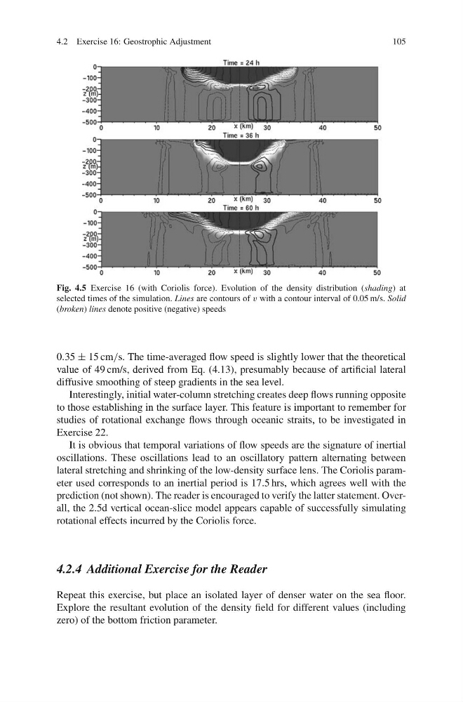
Fig. 4.5 Exercise 16 (with Coriolis force). Evolution of the density distribution (shading) at
selected times of the simulation. Lines are contours of v with a contour interval of 0.05 m/s. Solid
(broken) lines denote positive (negative) speeds
0.35 ± 15 cm/s. The time-averaged flow speed is slightly lower that the theoretical
value of 49 cm/s, derived from Eq. (4.13), presumably because of artificial lateral
diffusive smoothing of steep gradients in the sea level.
Interestingly, initial water-column stretching creates deep flows running opposite
to those establishing in the surface layer. This feature is important to remember for
studies of rotational exchange flows through oceanic straits, to be investigated in
Exercise 22.
It is obvious that temporal variations of flow speeds are the signature of inertial
oscillations. These oscillations lead to an oscillatory pattern alternating between
lateral stretching and shrinking of the low-density surface lens. The Coriolis parameter used corresponds to an inertial period is 17.5 hrs, which agrees well with the
prediction (not shown). The reader is encouraged to verify the latter statement. Overall, the 2.5d vertical ocean-slice model appears capable of successfully simulating
rotational effects incurred by the Coriolis force.
4.2.4 Additional Exercise for the Reader
Repeat this exercise, but place an isolated layer of denser water on the sea floor.
Explore the resultant evolution of the density field for different values (including
zero) of the bottom friction parameter.
105
Fig. 4.5 Exercise 16 (with Coriolis force). Evolution of the density distribution (shading) at
selected times of the simulation. Lines are contours of v with a contour interval of 0.05 m/s. Solid
(broken) lines denote positive (negative) speeds
0.35 ± 15 cm/s. The time-averaged flow speed is slightly lower that the theoretical
value of 49 cm/s, derived from Eq. (4.13), presumably because of artificial lateral
diffusive smoothing of steep gradients in the sea level.
Interestingly, initial water-column stretching creates deep flows running opposite
to those establishing in the surface layer. This feature is important to remember for
studies of rotational exchange flows through oceanic straits, to be investigated in
Exercise 22.
It is obvious that temporal variations of flow speeds are the signature of inertial
oscillations. These oscillations lead to an oscillatory pattern alternating between
lateral stretching and shrinking of the low-density surface lens. The Coriolis parameter used corresponds to an inertial period is 17.5 hrs, which agrees well with the
prediction (not shown). The reader is encouraged to verify the latter statement. Overall, the 2.5d vertical ocean-slice model appears capable of successfully simulating
rotational effects incurred by the Coriolis force.
4.2.4 Additional Exercise for the Reader
Repeat this exercise, but place an isolated layer of denser water on the sea floor.
Explore the resultant evolution of the density field for different values (including
zero) of the bottom friction parameter.