

4.2 Exercise 16: Geostrophic Adjustment
103
• Step structures of the sea floor are block-type obstacles for the vertically integrated continuity equation. This leads to a bias of the dynamics of gravity waves
via partial reflection.
These shortcoming, arising when using z-coordinate models, are unfortunate and
can only be avoided with the choice of other coordinate systems (such as sigmacoordinate models) or model types (such as layer models).
4.2 Exercise 16: Geostrophic Adjustment
4.2.1 Aim
This exercise employs the 2.5d vertical ocean-slice model to study geostrophic
adjustment of a surface density front of infinite length.
4.2.2 Task Description
We consider a model domain, 50 km in length and 500 m in depth, resolved by a
lateral grid spacing of Δx = 500 m and a vertical grid spacing of Δz = 10 m.
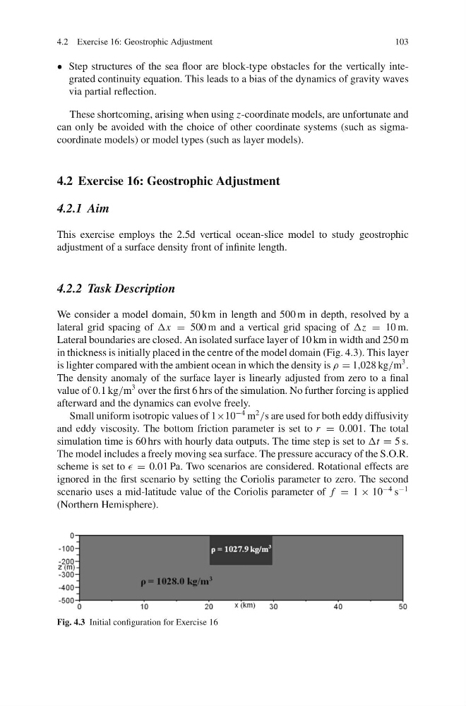
Lateral boundaries are closed. An isolated surface layer of 10 km in width and 250 m
in thickness is initially placed in the centre of the model domain (Fig. 4.3). This layer
is lighter compared with the ambient ocean in which the density is ρ = 1,028 kg/m
3 .
The density anomaly of the surface layer is linearly adjusted from zero to a final
value of 0.1 kg/m
3 over the first 6 hrs of the simulation. No further forcing is applied
afterward and the dynamics can evolve freely.
Small uniform isotropic values of 1×10
−4 m
2
/s are used for both eddy diffusivity
and eddy viscosity. The bottom friction parameter is set to r = 0.001. The total
simulation time is 60 hrs with hourly data outputs. The time step is set to Δt = 5 s.
The model includes a freely moving sea surface. The pressure accuracy of the S.O.R.
scheme is set to = 0.01 Pa. Two scenarios are considered. Rotational effects are
ignored in the first scenario by setting the Coriolis parameter to zero. The second
scenario uses a mid-latitude value of the Coriolis parameter of f = 1 × 10
−4 s
−1
(Northern Hemisphere).
Fig. 4.3 Initial configuration for Exercise 16
103
• Step structures of the sea floor are block-type obstacles for the vertically integrated continuity equation. This leads to a bias of the dynamics of gravity waves
via partial reflection.
These shortcoming, arising when using z-coordinate models, are unfortunate and
can only be avoided with the choice of other coordinate systems (such as sigmacoordinate models) or model types (such as layer models).
4.2 Exercise 16: Geostrophic Adjustment
4.2.1 Aim
This exercise employs the 2.5d vertical ocean-slice model to study geostrophic
adjustment of a surface density front of infinite length.
4.2.2 Task Description
We consider a model domain, 50 km in length and 500 m in depth, resolved by a
lateral grid spacing of Δx = 500 m and a vertical grid spacing of Δz = 10 m.
Lateral boundaries are closed. An isolated surface layer of 10 km in width and 250 m
in thickness is initially placed in the centre of the model domain (Fig. 4.3). This layer
is lighter compared with the ambient ocean in which the density is ρ = 1,028 kg/m
3 .
The density anomaly of the surface layer is linearly adjusted from zero to a final
value of 0.1 kg/m
3 over the first 6 hrs of the simulation. No further forcing is applied
afterward and the dynamics can evolve freely.
Small uniform isotropic values of 1×10
−4 m
2
/s are used for both eddy diffusivity
and eddy viscosity. The bottom friction parameter is set to r = 0.001. The total
simulation time is 60 hrs with hourly data outputs. The time step is set to Δt = 5 s.
The model includes a freely moving sea surface. The pressure accuracy of the S.O.R.
scheme is set to = 0.01 Pa. Two scenarios are considered. Rotational effects are
ignored in the first scenario by setting the Coriolis parameter to zero. The second
scenario uses a mid-latitude value of the Coriolis parameter of f = 1 × 10
−4 s
−1
(Northern Hemisphere).
Fig. 4.3 Initial configuration for Exercise 16