

102
4 2.5D Vertical Slice Modelling
u
∗
i,k = cos (α)u
n
i,k + sin (α)v
n
u + Δt F
n
u
v
n+1
i,k = cos (α)v
n
i,k − sin (α)u
n
v + Δt F
n
v
(4.16)
w
∗
i,k = w
n
i,k + Δt F
n
w
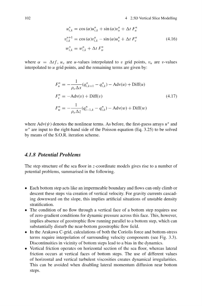
where α = Δt f , u v are u-values interpolated to v grid points, v u are v-values
interpolated to u grid points, and the remaining terms are given by:
F
n
u = −
1
ρ o Δx
(q
n
i,k+1 − q
n
i,k ) − Adv(u) + Diff(u)
F
n
v = −Adv(v) + Diff(v)
(4.17)
F
n
w = −
1
ρ o Δz
(q
n
i−1,k − q
n
i,k ) − Adv(w) + Diff(w)
where Adv(ψ) denotes the nonlinear terms. As before, the first-guess arrays u
∗ and
w
∗ are input to the right-hand side of the Poisson equation (Eq. 3.25) to be solved
by means of the S.O.R. iteration scheme.
4.1.8 Potential Problems
The step structure of the sea floor in z-coordinate models gives rise to a number of
potential problems, summarised in the following.
• Each bottom step acts like an impermeable boundary and flows can only climb or
descent these steps via creation of vertical velocity. For gravity currents cascading downward on the slope, this implies artificial situations of unstable density
stratification.
• The condition of no flow through a vertical face of a bottom step requires use
of zero-gradient conditions for dynamic pressure across this face. This, however,
implies absence of geostrophic flow running parallel to a bottom step, which can
substantially disturb the near-bottom geostrophic flow field.
• In the Arakawa C-grid, calculations of both the Coriolis force and bottom-stress
terms require interpolation of surrounding velocity components (see Fig. 3.3).
Discontinuities in vicinity of bottom steps lead to a bias in the dynamics.
• Vertical friction operates on horizontal section of the sea floor, whereas lateral
friction occurs at vertical faces of bottom steps. The use of different values
of horizontal and vertical turbulent viscosities creates dynamical irregularities.
This can be avoided when disabling lateral momentum diffusion near bottom
steps.
4 2.5D Vertical Slice Modelling
u
∗
i,k = cos (α)u
n
i,k + sin (α)v
n
u + Δt F
n
u
v
n+1
i,k = cos (α)v
n
i,k − sin (α)u
n
v + Δt F
n
v
(4.16)
w
∗
i,k = w
n
i,k + Δt F
n
w
where α = Δt f , u v are u-values interpolated to v grid points, v u are v-values
interpolated to u grid points, and the remaining terms are given by:
F
n
u = −
1
ρ o Δx
(q
n
i,k+1 − q
n
i,k ) − Adv(u) + Diff(u)
F
n
v = −Adv(v) + Diff(v)
(4.17)
F
n
w = −
1
ρ o Δz
(q
n
i−1,k − q
n
i,k ) − Adv(w) + Diff(w)
where Adv(ψ) denotes the nonlinear terms. As before, the first-guess arrays u
∗ and
w
∗ are input to the right-hand side of the Poisson equation (Eq. 3.25) to be solved
by means of the S.O.R. iteration scheme.
4.1.8 Potential Problems
The step structure of the sea floor in z-coordinate models gives rise to a number of
potential problems, summarised in the following.
• Each bottom step acts like an impermeable boundary and flows can only climb or
descent these steps via creation of vertical velocity. For gravity currents cascading downward on the slope, this implies artificial situations of unstable density
stratification.
• The condition of no flow through a vertical face of a bottom step requires use
of zero-gradient conditions for dynamic pressure across this face. This, however,
implies absence of geostrophic flow running parallel to a bottom step, which can
substantially disturb the near-bottom geostrophic flow field.
• In the Arakawa C-grid, calculations of both the Coriolis force and bottom-stress
terms require interpolation of surrounding velocity components (see Fig. 3.3).
Discontinuities in vicinity of bottom steps lead to a bias in the dynamics.
• Vertical friction operates on horizontal section of the sea floor, whereas lateral
friction occurs at vertical faces of bottom steps. The use of different values
of horizontal and vertical turbulent viscosities creates dynamical irregularities.
This can be avoided when disabling lateral momentum diffusion near bottom
steps.