

3.15 Turbulence
59
3.15.5 Turbulence Closure and Turbulent Diffusion
A turbulence closure is a mathematical expression that relates fluctuation of a variable to properties of the mean fl w. Some sort of turbulence closure is required in a
finite-di ference model, for we cannot resolve processes of periods shorter than the
time step or lengthscales smaller than the grid spacing.
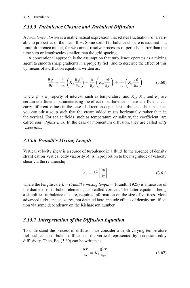
A conventional approach is the assumption that turbulence operates as a mixing
agent to smooth sharp gradients in a property fiel and to describe the effect of this
by means of a diffusion equation, written as:
∂ψ
∂t
=
∂
∂ x
K x
∂ψ
∂ x
+
∂
∂ y
K y
∂ψ
∂ y
+
∂
∂z
K z
∂ψ
∂z
(3.60)
where ψ is a property of interest, such as temperature, and K x , K y , and K z are
certain coefficient parameterising the effect of turbulence. These coefficient can
carry different values in the case of direction-dependent turbulence. For instance,
you can stir a soup such that the cream added mixes horizontally rather than in
the vertical. For scalar fields such as temperature or salinity, the coefficient are
called eddy diffusivities. In the case of momentum diffusion, they are called eddy
viscosities.
3.15.6 Prandtl’s Mixing Length
Vertical velocity shear is a source of turbulence in a fluid In the absence of density
stratification vertical eddy viscosity A z is in proportion to the magnitude of velocity
shear via the relationship:
A z = L
2
∂u
∂z
(3.61)
where the lengthscale L – Prandtl’s mixing length – (Prandtl, 1925) is a measure of
the diameter of turbulent elements, also called vortices. The latter equation, being
a simplifie turbulence closure, requires information on the size of vortices. More
advanced turbulence closures, not detailed here, include effects of density stratifica
tion via some dependency on the Richardson number.
3.15.7 Interpretation of the Diffusion Equation
To understand the process of diffusion, we consider a depth-varying temperature
fiel subject to turbulent diffusion in the vertical represented by a constant eddy
diffusivity. Then, Eq. (3.60) can be written as:
∂ T
∂t
= K z
∂
2
T
∂z 2
(3.62)
59
3.15.5 Turbulence Closure and Turbulent Diffusion
A turbulence closure is a mathematical expression that relates fluctuation of a variable to properties of the mean fl w. Some sort of turbulence closure is required in a
finite-di ference model, for we cannot resolve processes of periods shorter than the
time step or lengthscales smaller than the grid spacing.
A conventional approach is the assumption that turbulence operates as a mixing
agent to smooth sharp gradients in a property fiel and to describe the effect of this
by means of a diffusion equation, written as:
∂ψ
∂t
=
∂
∂ x
K x
∂ψ
∂ x
+
∂
∂ y
K y
∂ψ
∂ y
+
∂
∂z
K z
∂ψ
∂z
(3.60)
where ψ is a property of interest, such as temperature, and K x , K y , and K z are
certain coefficient parameterising the effect of turbulence. These coefficient can
carry different values in the case of direction-dependent turbulence. For instance,
you can stir a soup such that the cream added mixes horizontally rather than in
the vertical. For scalar fields such as temperature or salinity, the coefficient are
called eddy diffusivities. In the case of momentum diffusion, they are called eddy
viscosities.
3.15.6 Prandtl’s Mixing Length
Vertical velocity shear is a source of turbulence in a fluid In the absence of density
stratification vertical eddy viscosity A z is in proportion to the magnitude of velocity
shear via the relationship:
A z = L
2
∂u
∂z
(3.61)
where the lengthscale L – Prandtl’s mixing length – (Prandtl, 1925) is a measure of
the diameter of turbulent elements, also called vortices. The latter equation, being
a simplifie turbulence closure, requires information on the size of vortices. More
advanced turbulence closures, not detailed here, include effects of density stratifica
tion via some dependency on the Richardson number.
3.15.7 Interpretation of the Diffusion Equation
To understand the process of diffusion, we consider a depth-varying temperature
fiel subject to turbulent diffusion in the vertical represented by a constant eddy
diffusivity. Then, Eq. (3.60) can be written as:
∂ T
∂t
= K z
∂
2
T
∂z 2
(3.62)