

60
3 Basics of Geophysical Fluid Dynamics
This equation implies that the temperature will locally change as long as the temperature profil is curved. In other words, the temperature distribution approaches
a steady state once the a uniform vertical gradient in temperature is established
in the flui column. The value of turbulent diffusivity K z determines the time it
takes for this steady state to establish. Obviously, the resultant vertical temperature
gradient depends crucially on heat flu es across boundaries. In the absence of such
heat flu es, the steady-state temperature fiel can only be uniform (well-mixed)
throughout the fluid
3.16 The Navier–Stokes Equations
3.16.1 Complete Set of Equations
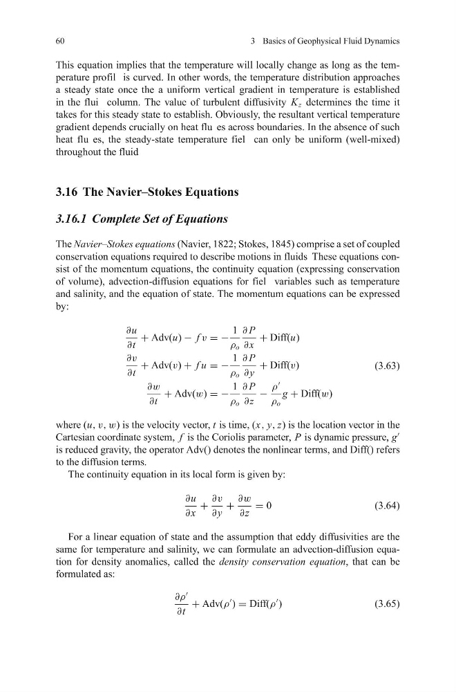
The Navier–Stokes equations (Navier, 1822; Stokes, 1845) comprise a set of coupled
conservation equations required to describe motions in fluids These equations consist of the momentum equations, the continuity equation (expressing conservation
of volume), advection-diffusion equations for fiel variables such as temperature
and salinity, and the equation of state. The momentum equations can be expressed
by:
∂u
∂t
+ Adv(u) − f v = −
1
ρ o
∂ P
∂ x
+ Diff(u)
∂v
∂t
+ Adv(v) + f u = −
1
ρ o
∂ P
∂ y
+ Diff(v)
∂w
∂t
+ Adv(w) = −
1
ρ o
∂ P
∂z
−
ρ
ρ o
g + Diff(w)
(3.63)
where (u, v, w) is the velocity vector, t is time, (x, y, z) is the location vector in the
Cartesian coordinate system, f is the Coriolis parameter, P is dynamic pressure, g
is reduced gravity, the operator Adv() denotes the nonlinear terms, and Diff() refers
to the diffusion terms.
The continuity equation in its local form is given by:
∂u
∂ x
+
∂v
∂ y
+
∂w
∂z
= 0
(3.64)
For a linear equation of state and the assumption that eddy diffusivities are the
same for temperature and salinity, we can formulate an advection-diffusion equation for density anomalies, called the density conservation equation, that can be
formulated as:
∂ρ
∂t
+ Adv(ρ
) = Diff(ρ
)
(3.65)
3 Basics of Geophysical Fluid Dynamics
This equation implies that the temperature will locally change as long as the temperature profil is curved. In other words, the temperature distribution approaches
a steady state once the a uniform vertical gradient in temperature is established
in the flui column. The value of turbulent diffusivity K z determines the time it
takes for this steady state to establish. Obviously, the resultant vertical temperature
gradient depends crucially on heat flu es across boundaries. In the absence of such
heat flu es, the steady-state temperature fiel can only be uniform (well-mixed)
throughout the fluid
3.16 The Navier–Stokes Equations
3.16.1 Complete Set of Equations
The Navier–Stokes equations (Navier, 1822; Stokes, 1845) comprise a set of coupled
conservation equations required to describe motions in fluids These equations consist of the momentum equations, the continuity equation (expressing conservation
of volume), advection-diffusion equations for fiel variables such as temperature
and salinity, and the equation of state. The momentum equations can be expressed
by:
∂u
∂t
+ Adv(u) − f v = −
1
ρ o
∂ P
∂ x
+ Diff(u)
∂v
∂t
+ Adv(v) + f u = −
1
ρ o
∂ P
∂ y
+ Diff(v)
∂w
∂t
+ Adv(w) = −
1
ρ o
∂ P
∂z
−
ρ
ρ o
g + Diff(w)
(3.63)
where (u, v, w) is the velocity vector, t is time, (x, y, z) is the location vector in the
Cartesian coordinate system, f is the Coriolis parameter, P is dynamic pressure, g
is reduced gravity, the operator Adv() denotes the nonlinear terms, and Diff() refers
to the diffusion terms.
The continuity equation in its local form is given by:
∂u
∂ x
+
∂v
∂ y
+
∂w
∂z
= 0
(3.64)
For a linear equation of state and the assumption that eddy diffusivities are the
same for temperature and salinity, we can formulate an advection-diffusion equation for density anomalies, called the density conservation equation, that can be
formulated as:
∂ρ
∂t
+ Adv(ρ
) = Diff(ρ
)
(3.65)