

164
6 Rotational Effects
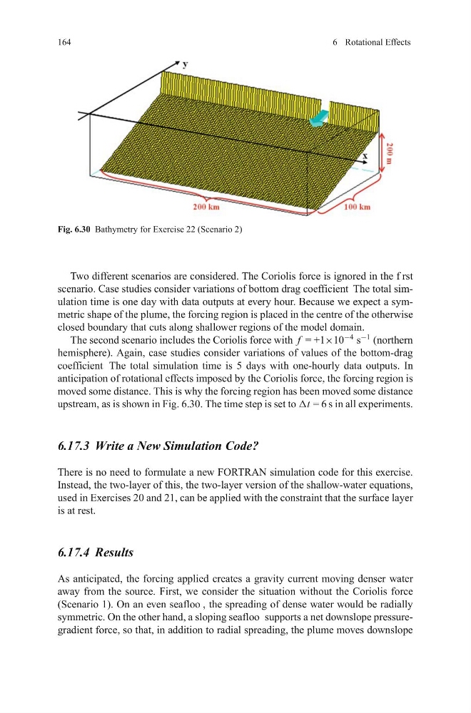
Fig. 6.30 Bathymetry for Exercise 22 (Scenario 2)
Two different scenarios are considered. The Coriolis force is ignored in the f rst
scenario. Case studies consider variations of bottom drag coefficient The total simulation time is one day with data outputs at every hour. Because we expect a symmetric shape of the plume, the forcing region is placed in the centre of the otherwise
closed boundary that cuts along shallower regions of the model domain.
The second scenario includes the Coriolis force with f = +1×10
−4
s
−1
(northern
hemisphere). Again, case studies consider variations of values of the bottom-drag
coefficient The total simulation time is 5 days with one-hourly data outputs. In
anticipation of rotational effects imposed by the Coriolis force, the forcing region is
moved some distance. This is why the forcing region has been moved some distance
upstream, as is shown in Fig. 6.30. The time step is set to Δt = 6 s in all experiments.
6.17.3 Write a New Simulation Code?
There is no need to formulate a new FORTRAN simulation code for this exercise.
Instead, the two-layer of this, the two-layer version of the shallow-water equations,
used in Exercises 20 and 21, can be applied with the constraint that the surface layer
is at rest.
6.17.4 Results
As anticipated, the forcing applied creates a gravity current moving denser water
away from the source. First, we consider the situation without the Coriolis force
(Scenario 1). On an even seafloo , the spreading of dense water would be radially
symmetric. On the other hand, a sloping seafloo supports a net downslope pressuregradient force, so that, in addition to radial spreading, the plume moves downslope
6 Rotational Effects
Fig. 6.30 Bathymetry for Exercise 22 (Scenario 2)
Two different scenarios are considered. The Coriolis force is ignored in the f rst
scenario. Case studies consider variations of bottom drag coefficient The total simulation time is one day with data outputs at every hour. Because we expect a symmetric shape of the plume, the forcing region is placed in the centre of the otherwise
closed boundary that cuts along shallower regions of the model domain.
The second scenario includes the Coriolis force with f = +1×10
−4
s
−1
(northern
hemisphere). Again, case studies consider variations of values of the bottom-drag
coefficient The total simulation time is 5 days with one-hourly data outputs. In
anticipation of rotational effects imposed by the Coriolis force, the forcing region is
moved some distance. This is why the forcing region has been moved some distance
upstream, as is shown in Fig. 6.30. The time step is set to Δt = 6 s in all experiments.
6.17.3 Write a New Simulation Code?
There is no need to formulate a new FORTRAN simulation code for this exercise.
Instead, the two-layer of this, the two-layer version of the shallow-water equations,
used in Exercises 20 and 21, can be applied with the constraint that the surface layer
is at rest.
6.17.4 Results
As anticipated, the forcing applied creates a gravity current moving denser water
away from the source. First, we consider the situation without the Coriolis force
(Scenario 1). On an even seafloo , the spreading of dense water would be radially
symmetric. On the other hand, a sloping seafloo supports a net downslope pressuregradient force, so that, in addition to radial spreading, the plume moves downslope