

6.17 Exercise 22: Reduced-Gravity Plumes
163
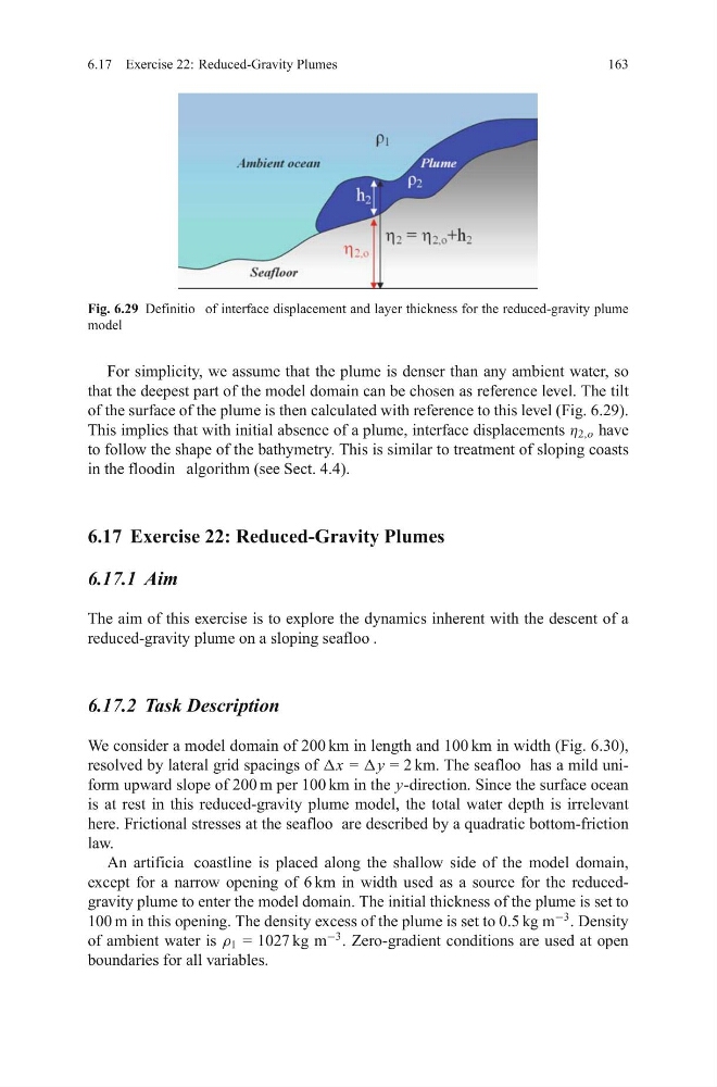
Fig. 6.29 Definitio of interface displacement and layer thickness for the reduced-gravity plume
model
For simplicity, we assume that the plume is denser than any ambient water, so
that the deepest part of the model domain can be chosen as reference level. The tilt
of the surface of the plume is then calculated with reference to this level (Fig. 6.29).
This implies that with initial absence of a plume, interface displacements η 2,o have
to follow the shape of the bathymetry. This is similar to treatment of sloping coasts
in the floodin algorithm (see Sect. 4.4).
6.17 Exercise 22: Reduced-Gravity Plumes
6.17.1 Aim
The aim of this exercise is to explore the dynamics inherent with the descent of a
reduced-gravity plume on a sloping seafloo .
6.17.2 Task Description
We consider a model domain of 200 km in length and 100 km in width (Fig. 6.30),
resolved by lateral grid spacings of Δx = Δy = 2 km. The seafloo has a mild uniform upward slope of 200 m per 100 km in the y-direction. Since the surface ocean
is at rest in this reduced-gravity plume model, the total water depth is irrelevant
here. Frictional stresses at the seafloo are described by a quadratic bottom-friction
law.
An artificia coastline is placed along the shallow side of the model domain,
except for a narrow opening of 6 km in width used as a source for the reducedgravity plume to enter the model domain. The initial thickness of the plume is set to
100 m in this opening. The density excess of the plume is set to 0.5 kg m
−3
. Density
of ambient water is ρ 1 = 1027 kg m
−3
. Zero-gradient conditions are used at open
boundaries for all variables.
163
Fig. 6.29 Definitio of interface displacement and layer thickness for the reduced-gravity plume
model
For simplicity, we assume that the plume is denser than any ambient water, so
that the deepest part of the model domain can be chosen as reference level. The tilt
of the surface of the plume is then calculated with reference to this level (Fig. 6.29).
This implies that with initial absence of a plume, interface displacements η 2,o have
to follow the shape of the bathymetry. This is similar to treatment of sloping coasts
in the floodin algorithm (see Sect. 4.4).
6.17 Exercise 22: Reduced-Gravity Plumes
6.17.1 Aim
The aim of this exercise is to explore the dynamics inherent with the descent of a
reduced-gravity plume on a sloping seafloo .
6.17.2 Task Description
We consider a model domain of 200 km in length and 100 km in width (Fig. 6.30),
resolved by lateral grid spacings of Δx = Δy = 2 km. The seafloo has a mild uniform upward slope of 200 m per 100 km in the y-direction. Since the surface ocean
is at rest in this reduced-gravity plume model, the total water depth is irrelevant
here. Frictional stresses at the seafloo are described by a quadratic bottom-friction
law.
An artificia coastline is placed along the shallow side of the model domain,
except for a narrow opening of 6 km in width used as a source for the reducedgravity plume to enter the model domain. The initial thickness of the plume is set to
100 m in this opening. The density excess of the plume is set to 0.5 kg m
−3
. Density
of ambient water is ρ 1 = 1027 kg m
−3
. Zero-gradient conditions are used at open
boundaries for all variables.