

146
6 Rotational Effects
and uniform lateral eddy viscosity with a value of A h = 500 m
2
/s. Bottom friction
is disabled.
6.9.3 Results
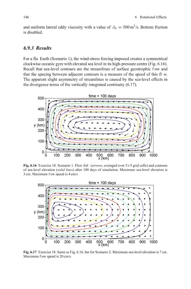
For a fla Earth (Scenario 1), the wind-stress forcing imposed creates a symmetrical
clockwise oceanic gyre with elevated sea level in its high-pressure centre (Fig. 6.16).
Recall that sea-level contours are the streamlines of surface geostrophic f ow and
that the spacing between adjacent contours is a measure of the speed of this fl w.
The apparent slight asymmetry of streamlines is caused by the sea-level effects in
the divergence terms of the vertically integrated continuity (6.17).
Fig. 6.16 Exercise 18. Scenario 1. Flow fiel (arrows, averaged over 5×5 grid cells) and contours
of sea-level elevation (solid lines) after 100 days of simulation. Maximum sea-level elevation is
3 cm. Maximum f ow speed is 4 cm/s
Fig. 6.17 Exercise 18. Same as Fig. 6.16, but for Scenario 2. Maximum sea-level elevation is 7 cm.
Maximum f ow speed is 20 cm/s
6 Rotational Effects
and uniform lateral eddy viscosity with a value of A h = 500 m
2
/s. Bottom friction
is disabled.
6.9.3 Results
For a fla Earth (Scenario 1), the wind-stress forcing imposed creates a symmetrical
clockwise oceanic gyre with elevated sea level in its high-pressure centre (Fig. 6.16).
Recall that sea-level contours are the streamlines of surface geostrophic f ow and
that the spacing between adjacent contours is a measure of the speed of this fl w.
The apparent slight asymmetry of streamlines is caused by the sea-level effects in
the divergence terms of the vertically integrated continuity (6.17).
Fig. 6.16 Exercise 18. Scenario 1. Flow fiel (arrows, averaged over 5×5 grid cells) and contours
of sea-level elevation (solid lines) after 100 days of simulation. Maximum sea-level elevation is
3 cm. Maximum f ow speed is 4 cm/s
Fig. 6.17 Exercise 18. Same as Fig. 6.16, but for Scenario 2. Maximum sea-level elevation is 7 cm.
Maximum f ow speed is 20 cm/s