

6.9 Exercise 18: The Wind-Driven Circulation
145
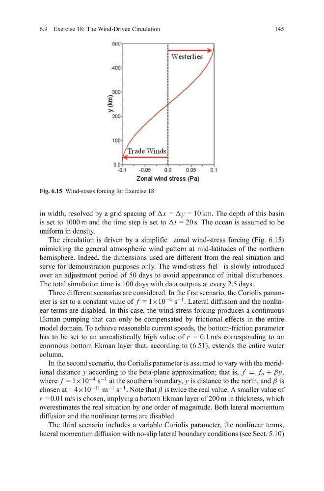
Fig. 6.15 Wind-stress forcing for Exercise 18
in width, resolved by a grid spacing of Δx = Δy = 10 km. The depth of this basin
is set to 1000 m and the time step is set to Δt = 20 s. The ocean is assumed to be
uniform in density.
The circulation is driven by a simplifie zonal wind-stress forcing (Fig. 6.15)
mimicking the general atmospheric wind pattern at mid-latitudes of the northern
hemisphere. Indeed, the dimensions used are different from the real situation and
serve for demonstration purposes only. The wind-stress fiel is slowly introduced
over an adjustment period of 50 days to avoid appearance of initial disturbances.
The total simulation time is 100 days with data outputs at every 2.5 days.
Three different scenarios are considered. In the f rst scenario, the Coriolis parameter is set to a constant value of f = 1×10
−4
s
−1
. Lateral diffusion and the nonlinear terms are disabled. In this case, the wind-stress forcing produces a continuous
Ekman pumping that can only be compensated by frictional effects in the entire
model domain. To achieve reasonable current speeds, the bottom-friction parameter
has to be set to an unrealistically high value of r = 0.1 m/s corresponding to an
enormous bottom Ekman layer that, according to (6.51), extends the entire water
column.
In the second scenario, the Coriolis parameter is assumed to vary with the meridional distance y according to the beta-plane approximation; that is, f = f o + βy,
where f = 1×10
−4
s
−1
at the southern boundary, y is distance to the north, and β is
chosen at = 4×10
−11
m
−1
s
−1
. Note that β is twice the real value. A smaller value of
r = 0.01 m/s is chosen, implying a bottom Ekman layer of 200 m in thickness, which
overestimates the real situation by one order of magnitude. Both lateral momentum
diffusion and the nonlinear terms are disabled.
The third scenario includes a variable Coriolis parameter, the nonlinear terms,
lateral momentum diffusion with no-slip lateral boundary conditions (see Sect. 5.10)
145
Fig. 6.15 Wind-stress forcing for Exercise 18
in width, resolved by a grid spacing of Δx = Δy = 10 km. The depth of this basin
is set to 1000 m and the time step is set to Δt = 20 s. The ocean is assumed to be
uniform in density.
The circulation is driven by a simplifie zonal wind-stress forcing (Fig. 6.15)
mimicking the general atmospheric wind pattern at mid-latitudes of the northern
hemisphere. Indeed, the dimensions used are different from the real situation and
serve for demonstration purposes only. The wind-stress fiel is slowly introduced
over an adjustment period of 50 days to avoid appearance of initial disturbances.
The total simulation time is 100 days with data outputs at every 2.5 days.
Three different scenarios are considered. In the f rst scenario, the Coriolis parameter is set to a constant value of f = 1×10
−4
s
−1
. Lateral diffusion and the nonlinear terms are disabled. In this case, the wind-stress forcing produces a continuous
Ekman pumping that can only be compensated by frictional effects in the entire
model domain. To achieve reasonable current speeds, the bottom-friction parameter
has to be set to an unrealistically high value of r = 0.1 m/s corresponding to an
enormous bottom Ekman layer that, according to (6.51), extends the entire water
column.
In the second scenario, the Coriolis parameter is assumed to vary with the meridional distance y according to the beta-plane approximation; that is, f = f o + βy,
where f = 1×10
−4
s
−1
at the southern boundary, y is distance to the north, and β is
chosen at = 4×10
−11
m
−1
s
−1
. Note that β is twice the real value. A smaller value of
r = 0.01 m/s is chosen, implying a bottom Ekman layer of 200 m in thickness, which
overestimates the real situation by one order of magnitude. Both lateral momentum
diffusion and the nonlinear terms are disabled.
The third scenario includes a variable Coriolis parameter, the nonlinear terms,
lateral momentum diffusion with no-slip lateral boundary conditions (see Sect. 5.10)