

6.8 The Wind-Driven Circulation of the Ocean
143
a f ow convergence/divergence in the bottom Ekman layer. For consistency with the
analytical solution of the Ekman-layer equations (see Cushman-Roisin, 1994), the
linear friction parameter has to be chosen according to:
r = 0.5 δ ek f
(6.51)
where the Ekman-layer thickness is given by (6.43).
6.8.10 Western Boundary Currents
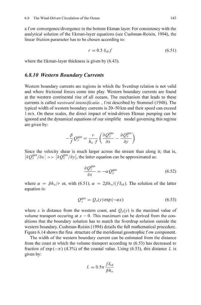
Western boundary currents are regions in which the Sverdrup relation is not valid
and where frictional forces come into play. Western boundary currents are found
at the western continental rise of all oceans. The mechanism that leads to these
currents is called westward intensificatio , f rst described by Stommel (1948). The
typical width of western boundary currents is 20–50 km and their speed can exceed
1 m/s. On these scales, the direct impact of wind-driven Ekman pumping can be
ignored and the dynamical equations of our simplifie model governing this regime
are given by:
−
β
f
Q
geo
y =
r
h o f
∂ Q
geo
y
∂ x
−
∂ Q
geo
x
∂ y
Since the velocity shear is much larger across the stream than along it; that is,
∂ Q
geo
y /∂ x
>>
∂ Q
geo
x /∂ y
, the latter equation can be approximated as:
∂ Q
geo
y
∂ x
= −α Q
geo
y
(6.52)
where α = βh o /r or, with (6.51), α = 2βh o /( f δ ek ). The solution of the latter
equation is:
Q
geo
y = Q o (y) exp (−αx)
(6.53)
where x is distance from the western coast, and Q o (y) is the maximal value of
volume transport occuring at x = 0. This maximum can be derived from the conditions that the boundary solution has to match the Sverdrup solution outside the
western boundary. Cushman-Roisin (1994) details the full mathematical procedure.
Figure 6.14 shows the fina structure of the meridional geostrophic f ow component.
The width of the western boundary current can be estimated from the distance
from the coast at which the volume transport according to (6.53) has decreased to
fraction of exp (−π ) (4.3%) of the coastal value. Using (6.53), this distance L is
given by:
L = 0.5π
f δ ek
βh o
143
a f ow convergence/divergence in the bottom Ekman layer. For consistency with the
analytical solution of the Ekman-layer equations (see Cushman-Roisin, 1994), the
linear friction parameter has to be chosen according to:
r = 0.5 δ ek f
(6.51)
where the Ekman-layer thickness is given by (6.43).
6.8.10 Western Boundary Currents
Western boundary currents are regions in which the Sverdrup relation is not valid
and where frictional forces come into play. Western boundary currents are found
at the western continental rise of all oceans. The mechanism that leads to these
currents is called westward intensificatio , f rst described by Stommel (1948). The
typical width of western boundary currents is 20–50 km and their speed can exceed
1 m/s. On these scales, the direct impact of wind-driven Ekman pumping can be
ignored and the dynamical equations of our simplifie model governing this regime
are given by:
−
β
f
Q
geo
y =
r
h o f
∂ Q
geo
y
∂ x
−
∂ Q
geo
x
∂ y
Since the velocity shear is much larger across the stream than along it; that is,
∂ Q
geo
y /∂ x
>>
∂ Q
geo
x /∂ y
, the latter equation can be approximated as:
∂ Q
geo
y
∂ x
= −α Q
geo
y
(6.52)
where α = βh o /r or, with (6.51), α = 2βh o /( f δ ek ). The solution of the latter
equation is:
Q
geo
y = Q o (y) exp (−αx)
(6.53)
where x is distance from the western coast, and Q o (y) is the maximal value of
volume transport occuring at x = 0. This maximum can be derived from the conditions that the boundary solution has to match the Sverdrup solution outside the
western boundary. Cushman-Roisin (1994) details the full mathematical procedure.
Figure 6.14 shows the fina structure of the meridional geostrophic f ow component.
The width of the western boundary current can be estimated from the distance
from the coast at which the volume transport according to (6.53) has decreased to
fraction of exp (−π ) (4.3%) of the coastal value. Using (6.53), this distance L is
given by:
L = 0.5π
f δ ek
βh o