

116
5 2D Shallow-Water Modelling
zero-slip condition. The semi-slip condition gives half the velocity shear compared
with the no-slip condition and it is realised by setting f ow at land grid points to
zero. Figure 5.17 illustrates these conditions.
5.10.6 Task Description
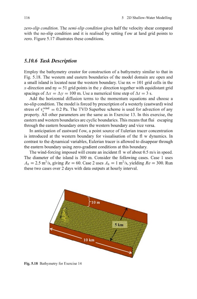
Employ the bathymetry creator for construction of a bathymetry similar to that in
Fig. 5.18. The western and eastern boundaries of the model domain are open and
a small island is located near the western boundary. Use nx = 101 grid cells in the
x-direction and ny = 51 grid points in the y direction together with equidistant grid
spacings of Δx = Δy = 100 m. Use a numerical time step of Δt = 3 s.
Add the horizontal diffusion terms to the momentum equations and choose a
no-slip condition. The model is forced by prescription of a westerly (eastward) wind
stress of τ
wind
x
= 0.2 Pa. The TVD Superbee scheme is used for advection of any
property. All other parameters are the same as in Exercise 13. In this exercise, the
eastern and western boundaries are cyclic boundaries. This means that flui escaping
through the eastern boundary enters the western boundary and vice versa.
In anticipation of eastward f ow, a point source of Eulerian tracer concentration
is introduced at the western boundary for visualisation of the fl w dynamics. In
contrast to the dynamical variables, Eulerian tracer is allowed to disappear through
the eastern boundary using zero-gradient conditions at this boundary.
The wind-forcing imposed will create an incident fl w of about 0.5 m/s in speed.
The diameter of the island is 300 m. Consider the following cases. Case 1 uses
A h = 2.5 m
2
/s, giving Re = 60. Case 2 uses A h = 1 m
2
/s, yielding Re = 300. Run
these two cases over 2 days with data outputs at hourly interval.
Fig. 5.18 Bathymetry for Exercise 14
5 2D Shallow-Water Modelling
zero-slip condition. The semi-slip condition gives half the velocity shear compared
with the no-slip condition and it is realised by setting f ow at land grid points to
zero. Figure 5.17 illustrates these conditions.
5.10.6 Task Description
Employ the bathymetry creator for construction of a bathymetry similar to that in
Fig. 5.18. The western and eastern boundaries of the model domain are open and
a small island is located near the western boundary. Use nx = 101 grid cells in the
x-direction and ny = 51 grid points in the y direction together with equidistant grid
spacings of Δx = Δy = 100 m. Use a numerical time step of Δt = 3 s.
Add the horizontal diffusion terms to the momentum equations and choose a
no-slip condition. The model is forced by prescription of a westerly (eastward) wind
stress of τ
wind
x
= 0.2 Pa. The TVD Superbee scheme is used for advection of any
property. All other parameters are the same as in Exercise 13. In this exercise, the
eastern and western boundaries are cyclic boundaries. This means that flui escaping
through the eastern boundary enters the western boundary and vice versa.
In anticipation of eastward f ow, a point source of Eulerian tracer concentration
is introduced at the western boundary for visualisation of the fl w dynamics. In
contrast to the dynamical variables, Eulerian tracer is allowed to disappear through
the eastern boundary using zero-gradient conditions at this boundary.
The wind-forcing imposed will create an incident fl w of about 0.5 m/s in speed.
The diameter of the island is 300 m. Consider the following cases. Case 1 uses
A h = 2.5 m
2
/s, giving Re = 60. Case 2 uses A h = 1 m
2
/s, yielding Re = 300. Run
these two cases over 2 days with data outputs at hourly interval.
Fig. 5.18 Bathymetry for Exercise 14