

92
5 2D Shallow-Water Modelling
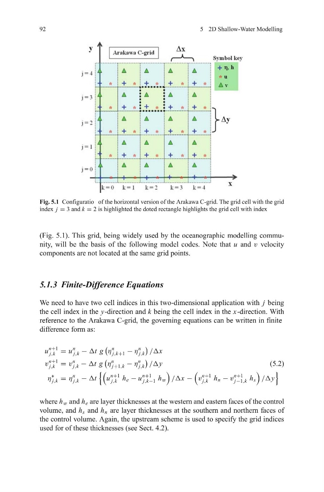
Fig. 5.1 Configuratio of the horizontal version of the Arakawa C-grid. The grid cell with the grid
index j = 3 and k = 2 is highlighted the doted rectangle highlights the grid cell with index
(Fig. 5.1). This grid, being widely used by the oceanographic modelling community, will be the basis of the following model codes. Note that u and v velocity
components are not located at the same grid points.
5.1.3 Finite-Difference Equations
We need to have two cell indices in this two-dimensional application with j being
the cell index in the y-direction and k being the cell index in the x-direction. With
reference to the Arakawa C-grid, the governing equations can be written in finite
difference form as:
u
n+1
j,k = u
n
j,k − Δt g
η
n
j,k+1 − η
n
j,k
/Δx
v
n+1
j,k = v
n
j,k − Δt g
η
n
j+1,k − η
n
j,k
/Δy
(5.2)
η
∗
j,k = η
n
j,k − Δt
u
n+1
j,k h e − u
n+1
j,k−1 h w
/Δx −
v
n+1
j,k h n − v
n+1
j−1,k h s
/Δy
where h w and h e are layer thicknesses at the western and eastern faces of the control
volume, and h s and h n are layer thicknesses at the southern and northern faces of
the control volume. Again, the upstream scheme is used to specify the grid indices
used for of these thicknesses (see Sect. 4.2).
5 2D Shallow-Water Modelling
Fig. 5.1 Configuratio of the horizontal version of the Arakawa C-grid. The grid cell with the grid
index j = 3 and k = 2 is highlighted the doted rectangle highlights the grid cell with index
(Fig. 5.1). This grid, being widely used by the oceanographic modelling community, will be the basis of the following model codes. Note that u and v velocity
components are not located at the same grid points.
5.1.3 Finite-Difference Equations
We need to have two cell indices in this two-dimensional application with j being
the cell index in the y-direction and k being the cell index in the x-direction. With
reference to the Arakawa C-grid, the governing equations can be written in finite
difference form as:
u
n+1
j,k = u
n
j,k − Δt g
η
n
j,k+1 − η
n
j,k
/Δx
v
n+1
j,k = v
n
j,k − Δt g
η
n
j+1,k − η
n
j,k
/Δy
(5.2)
η
∗
j,k = η
n
j,k − Δt
u
n+1
j,k h e − u
n+1
j,k−1 h w
/Δx −
v
n+1
j,k h n − v
n+1
j−1,k h s
/Δy
where h w and h e are layer thicknesses at the western and eastern faces of the control
volume, and h s and h n are layer thicknesses at the southern and northern faces of
the control volume. Again, the upstream scheme is used to specify the grid indices
used for of these thicknesses (see Sect. 4.2).