

5.1 Long Waves in a Shallow Lake
93
In addition to this, sea-level elevations are slightly smoothed with use of the twodimensional version of the first-orde Shapiro filte . To this end, values of sea-level
elevation for the next time level follow from:
η
n+1
j,k = (1 − )η
∗
j,k + 0.25
η
∗
j,k−1 + η
∗
j,k+1 + η
∗
j−1,k + η
∗
j+1,k
(5.3)
The parameter determines the degree of smoothing.
5.1.4 Inclusion of Land and Coastlines
As in the 1D shallow water model, water-depth values determine whether gridpoints
belong to the ocean or to the land and also the location of coastlines. Land is here
define as zero or negative values of water depth and velocity components are kept
at zero values in these “dry” grid cells during a simulation. Coastlines are implicitly
define by setting the fl w component normal to a coastline to zero. Owing to the
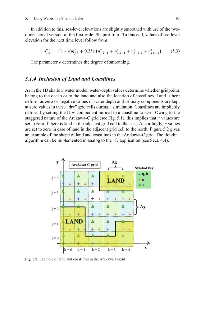
staggered nature of the Arakawa-C grid (see Fig. 5.1), this implies that u values are
set to zero if there is land in the adjacent grid cell to the east. Accordingly, v values
are set to zero in case of land in the adjacent grid cell to the north. Figure 5.2 gives
an example of the shape of land and coastlines in the Arakawa-C grid. The floodin
algorithm can be implemented in analog to the 1D application (see Sect. 4.4).
Fig. 5.2 Example of land and coastlines in the Arakawa C-grid
93
In addition to this, sea-level elevations are slightly smoothed with use of the twodimensional version of the first-orde Shapiro filte . To this end, values of sea-level
elevation for the next time level follow from:
η
n+1
j,k = (1 − )η
∗
j,k + 0.25
η
∗
j,k−1 + η
∗
j,k+1 + η
∗
j−1,k + η
∗
j+1,k
(5.3)
The parameter determines the degree of smoothing.
5.1.4 Inclusion of Land and Coastlines
As in the 1D shallow water model, water-depth values determine whether gridpoints
belong to the ocean or to the land and also the location of coastlines. Land is here
define as zero or negative values of water depth and velocity components are kept
at zero values in these “dry” grid cells during a simulation. Coastlines are implicitly
define by setting the fl w component normal to a coastline to zero. Owing to the
staggered nature of the Arakawa-C grid (see Fig. 5.1), this implies that u values are
set to zero if there is land in the adjacent grid cell to the east. Accordingly, v values
are set to zero in case of land in the adjacent grid cell to the north. Figure 5.2 gives
an example of the shape of land and coastlines in the Arakawa-C grid. The floodin
algorithm can be implemented in analog to the 1D application (see Sect. 4.4).
Fig. 5.2 Example of land and coastlines in the Arakawa C-grid