

Chapter 5
2D Shallow-Water Modelling
Abstract This chapter applies the two-dimensional shallow-water equations to
study various processes such as surface gravity waves, the wind-driven circulation
in a lake, the formation of turbulent island wakes, and the barotropic instability
mechanism. The reader is introduced to various advection schemes simulating the
movement of Eulerian tracer and describing the nonlinear terms in the momentum
equations.
5.1 Long Waves in a Shallow Lake
5.1.1 The 2D Shallow-Water Wave Equations
We assume a lake of uniform water density and allow for variable bathymetry. For
simplicity, frictional effects and the coriolis force are ignored and so are the nonlinear terms. This implies that our waves have a period short compared with the inertial
period and that the phase speed of waves exceeds fl w speeds by far. Under these
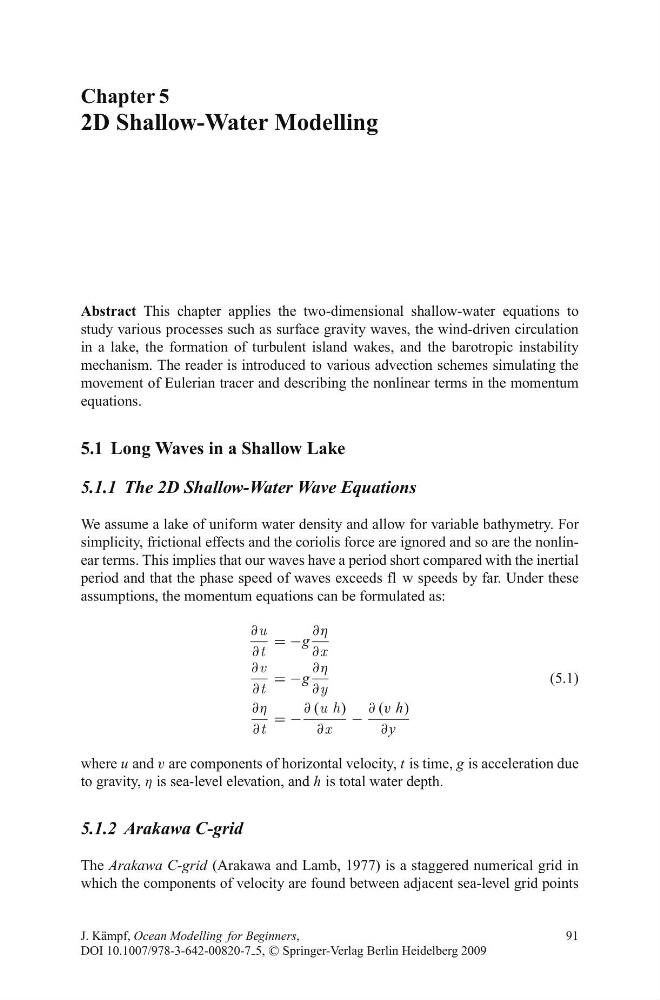
assumptions, the momentum equations can be formulated as:
∂u
∂t
= −g
∂η
∂x
∂v
∂t
= −g
∂η
∂y
(5.1)
∂η
∂t
= −
∂ (u h)
∂x
−
∂ (v h)
∂ y
where u and v are components of horizontal velocity, t is time, g is acceleration due
to gravity, η is sea-level elevation, and h is total water depth.
5.1.2 Arakawa C-grid
The Arakawa C-grid (Arakawa and Lamb, 1977) is a staggered numerical grid in
which the components of velocity are found between adjacent sea-level grid points
J. K¨ ampf, Ocean Modelling for Beginners,
DOI 10.1007/978-3-642-00820-7 5, C
Springer-Verlag Berlin Heidelberg 2009
91
2D Shallow-Water Modelling
Abstract This chapter applies the two-dimensional shallow-water equations to
study various processes such as surface gravity waves, the wind-driven circulation
in a lake, the formation of turbulent island wakes, and the barotropic instability
mechanism. The reader is introduced to various advection schemes simulating the
movement of Eulerian tracer and describing the nonlinear terms in the momentum
equations.
5.1 Long Waves in a Shallow Lake
5.1.1 The 2D Shallow-Water Wave Equations
We assume a lake of uniform water density and allow for variable bathymetry. For
simplicity, frictional effects and the coriolis force are ignored and so are the nonlinear terms. This implies that our waves have a period short compared with the inertial
period and that the phase speed of waves exceeds fl w speeds by far. Under these
assumptions, the momentum equations can be formulated as:
∂u
∂t
= −g
∂η
∂x
∂v
∂t
= −g
∂η
∂y
(5.1)
∂η
∂t
= −
∂ (u h)
∂x
−
∂ (v h)
∂ y
where u and v are components of horizontal velocity, t is time, g is acceleration due
to gravity, η is sea-level elevation, and h is total water depth.
5.1.2 Arakawa C-grid
The Arakawa C-grid (Arakawa and Lamb, 1977) is a staggered numerical grid in
which the components of velocity are found between adjacent sea-level grid points
J. K¨ ampf, Ocean Modelling for Beginners,
DOI 10.1007/978-3-642-00820-7 5, C
Springer-Verlag Berlin Heidelberg 2009
91