

19 Forecasting the Coastal Optical Properties Using Satellite Ocean Color
341
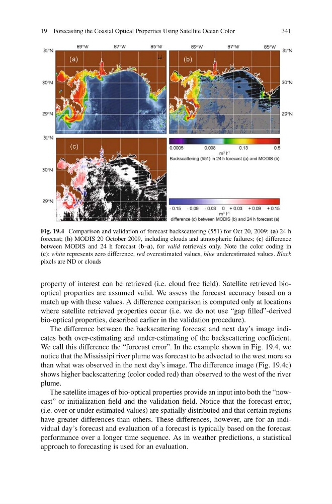
Fig. 19.4 Comparison and validation of forecast backscattering (551) for Oct 20, 2009: (a) 24 h
forecast; (b) MODIS 20 October 2009, including clouds and atmospheric failures; (c) difference
between MODIS and 24 h forecast (b–a), for valid retrievals only. Note the color coding in
(c): white represents zero difference, red overestimated values, blue underestimated values. Black
pixels are ND or clouds
property of interest can be retrieved (i.e. cloud free field). Satellite retrieved biooptical properties are assumed valid. We assess the forecast accuracy based on a
match up with these values. A difference comparison is computed only at locations
where satellite retrieved properties occur (i.e. we do not use “gap filled”-derived
bio-optical properties, described earlier in the validation procedure).
The difference between the backscattering forecast and next day’s image indicates both over-estimating and under-estimating of the backscattering coefficient.
We call this difference the “forecast error”. In the example shown in Fig. 19.4, we
notice that the Mississipi river plume was forecast to be advected to the west more so
than what was observed in the next day’s image. The difference image (Fig. 19.4c)
shows higher backscattering (color coded red) than observed to the west of the river
plume.
The satellite images of bio-optical properties provide an input into both the “nowcast” or initialization field and the validation field. Notice that the forecast error,
(i.e. over or under estimated values) are spatially distributed and that certain regions
have greater differences than others. These differences, however, are for an individual day’s forecast and evaluation of a forecast is typically based on the forecast
performance over a longer time sequence. As in weather predictions, a statistical
approach to forecasting is used for an evaluation.
341
Fig. 19.4 Comparison and validation of forecast backscattering (551) for Oct 20, 2009: (a) 24 h
forecast; (b) MODIS 20 October 2009, including clouds and atmospheric failures; (c) difference
between MODIS and 24 h forecast (b–a), for valid retrievals only. Note the color coding in
(c): white represents zero difference, red overestimated values, blue underestimated values. Black
pixels are ND or clouds
property of interest can be retrieved (i.e. cloud free field). Satellite retrieved biooptical properties are assumed valid. We assess the forecast accuracy based on a
match up with these values. A difference comparison is computed only at locations
where satellite retrieved properties occur (i.e. we do not use “gap filled”-derived
bio-optical properties, described earlier in the validation procedure).
The difference between the backscattering forecast and next day’s image indicates both over-estimating and under-estimating of the backscattering coefficient.
We call this difference the “forecast error”. In the example shown in Fig. 19.4, we
notice that the Mississipi river plume was forecast to be advected to the west more so
than what was observed in the next day’s image. The difference image (Fig. 19.4c)
shows higher backscattering (color coded red) than observed to the west of the river
plume.
The satellite images of bio-optical properties provide an input into both the “nowcast” or initialization field and the validation field. Notice that the forecast error,
(i.e. over or under estimated values) are spatially distributed and that certain regions
have greater differences than others. These differences, however, are for an individual day’s forecast and evaluation of a forecast is typically based on the forecast
performance over a longer time sequence. As in weather predictions, a statistical
approach to forecasting is used for an evaluation.