

10 Absolute Dynamic Topography from Altimetry
167
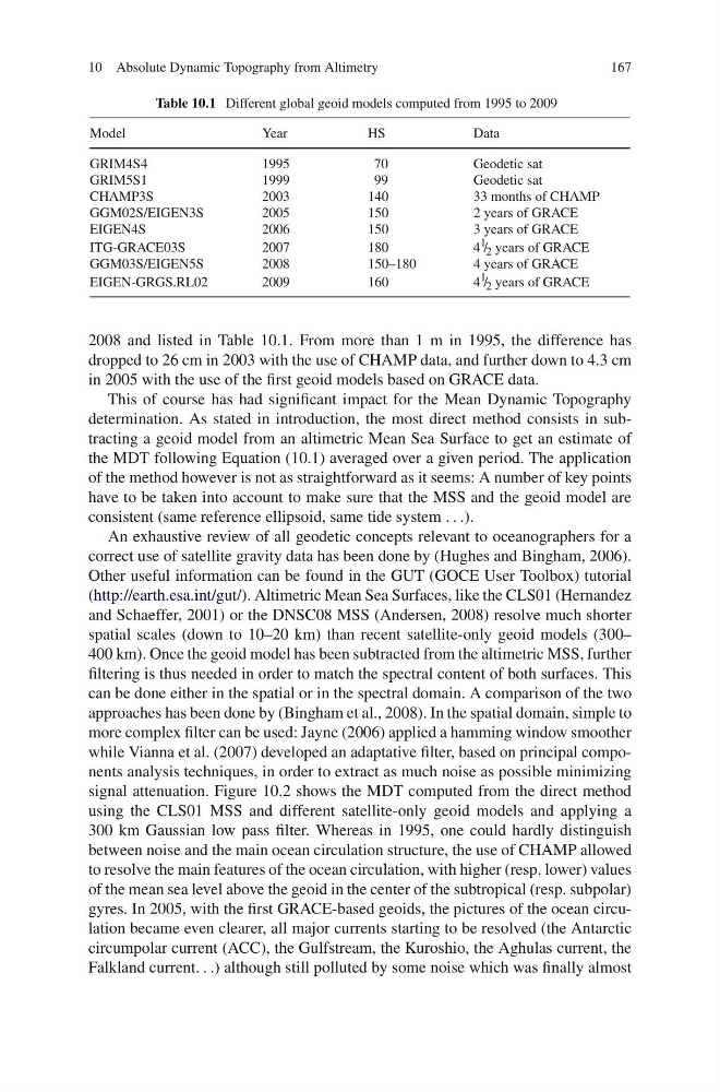
Table 10.1 Different global geoid models computed from 1995 to 2009
Model
Year
HS
Data
GRIM4S4
1995
70
Geodetic sat
GRIM5S1
1999
99
Geodetic sat
CHAMP3S
2003
140
33 months of CHAMP
GGM02S/EIGEN3S
2005
150
2 years of GRACE
EIGEN4S
2006
150
3 years of GRACE
ITG-GRACE03S
2007
180
4
1 / 2 years of GRACE
GGM03S/EIGEN5S
2008
150–180
4 years of GRACE
EIGEN-GRGS.RL02
2009
160
4
1
/ 2 years of GRACE
2008 and listed in Table 10.1. From more than 1 m in 1995, the difference has
dropped to 26 cm in 2003 with the use of CHAMP data, and further down to 4.3 cm
in 2005 with the use of the first geoid models based on GRACE data.
This of course has had significant impact for the Mean Dynamic Topography
determination. As stated in introduction, the most direct method consists in subtracting a geoid model from an altimetric Mean Sea Surface to get an estimate of
the MDT following Equation (10.1) averaged over a given period. The application
of the method however is not as straightforward as it seems: A number of key points
have to be taken into account to make sure that the MSS and the geoid model are
consistent (same reference ellipsoid, same tide system . . .).
An exhaustive review of all geodetic concepts relevant to oceanographers for a
correct use of satellite gravity data has been done by (Hughes and Bingham, 2006).
Other useful information can be found in the GUT (GOCE User Toolbox) tutorial
(http://earth.esa.int/gut/). Altimetric Mean Sea Surfaces, like the CLS01 (Hernandez
and Schaeffer, 2001) or the DNSC08 MSS (Andersen, 2008) resolve much shorter
spatial scales (down to 10–20 km) than recent satellite-only geoid models (300–
400 km). Once the geoid model has been subtracted from the altimetric MSS, further
filtering is thus needed in order to match the spectral content of both surfaces. This
can be done either in the spatial or in the spectral domain. A comparison of the two
approaches has been done by (Bingham et al., 2008). In the spatial domain, simple to
more complex filter can be used: Jayne (2006) applied a hamming window smoother
while Vianna et al. (2007) developed an adaptative filter, based on principal components analysis techniques, in order to extract as much noise as possible minimizing
signal attenuation. Figure 10.2 shows the MDT computed from the direct method
using the CLS01 MSS and different satellite-only geoid models and applying a
300 km Gaussian low pass filter. Whereas in 1995, one could hardly distinguish
between noise and the main ocean circulation structure, the use of CHAMP allowed
to resolve the main features of the ocean circulation, with higher (resp. lower) values
of the mean sea level above the geoid in the center of the subtropical (resp. subpolar)
gyres. In 2005, with the first GRACE-based geoids, the pictures of the ocean circulation became even clearer, all major currents starting to be resolved (the Antarctic
circumpolar current (ACC), the Gulfstream, the Kuroshio, the Aghulas current, the
Falkland current. . .) although still polluted by some noise which was finally almost
167
Table 10.1 Different global geoid models computed from 1995 to 2009
Model
Year
HS
Data
GRIM4S4
1995
70
Geodetic sat
GRIM5S1
1999
99
Geodetic sat
CHAMP3S
2003
140
33 months of CHAMP
GGM02S/EIGEN3S
2005
150
2 years of GRACE
EIGEN4S
2006
150
3 years of GRACE
ITG-GRACE03S
2007
180
4
1 / 2 years of GRACE
GGM03S/EIGEN5S
2008
150–180
4 years of GRACE
EIGEN-GRGS.RL02
2009
160
4
1
/ 2 years of GRACE
2008 and listed in Table 10.1. From more than 1 m in 1995, the difference has
dropped to 26 cm in 2003 with the use of CHAMP data, and further down to 4.3 cm
in 2005 with the use of the first geoid models based on GRACE data.
This of course has had significant impact for the Mean Dynamic Topography
determination. As stated in introduction, the most direct method consists in subtracting a geoid model from an altimetric Mean Sea Surface to get an estimate of
the MDT following Equation (10.1) averaged over a given period. The application
of the method however is not as straightforward as it seems: A number of key points
have to be taken into account to make sure that the MSS and the geoid model are
consistent (same reference ellipsoid, same tide system . . .).
An exhaustive review of all geodetic concepts relevant to oceanographers for a
correct use of satellite gravity data has been done by (Hughes and Bingham, 2006).
Other useful information can be found in the GUT (GOCE User Toolbox) tutorial
(http://earth.esa.int/gut/). Altimetric Mean Sea Surfaces, like the CLS01 (Hernandez
and Schaeffer, 2001) or the DNSC08 MSS (Andersen, 2008) resolve much shorter
spatial scales (down to 10–20 km) than recent satellite-only geoid models (300–
400 km). Once the geoid model has been subtracted from the altimetric MSS, further
filtering is thus needed in order to match the spectral content of both surfaces. This
can be done either in the spatial or in the spectral domain. A comparison of the two
approaches has been done by (Bingham et al., 2008). In the spatial domain, simple to
more complex filter can be used: Jayne (2006) applied a hamming window smoother
while Vianna et al. (2007) developed an adaptative filter, based on principal components analysis techniques, in order to extract as much noise as possible minimizing
signal attenuation. Figure 10.2 shows the MDT computed from the direct method
using the CLS01 MSS and different satellite-only geoid models and applying a
300 km Gaussian low pass filter. Whereas in 1995, one could hardly distinguish
between noise and the main ocean circulation structure, the use of CHAMP allowed
to resolve the main features of the ocean circulation, with higher (resp. lower) values
of the mean sea level above the geoid in the center of the subtropical (resp. subpolar)
gyres. In 2005, with the first GRACE-based geoids, the pictures of the ocean circulation became even clearer, all major currents starting to be resolved (the Antarctic
circumpolar current (ACC), the Gulfstream, the Kuroshio, the Aghulas current, the
Falkland current. . .) although still polluted by some noise which was finally almost