

4. The mean of the reduced gravity data (steps 1-3) is then subtracted to center the data
for each computational cell before covariance and mean anomaly calculations.
After these 4 steps the L vector in (3a) is complete.
5. Develop accurate covariance models (Heiskanen and Moritz, 1967) of local, reduced
gravity fields in 1 Ox 1 ° cells with a 30' overlap. The convergence of the meridians in high
latitudes is compensated for by extending the East-West overlap around each 1 °xl ° cell
using the cosine of the latitude. For example, between -30° S and 30° N the overlap is 30'
but from 50° to 60° N the overlap is 45' East-West; 60° to 70° - overlap 60'; 70° to 80° -
overlap 90'; and 80° to 90° - overlap 180'. The covariance defines the statistical
correlation of gravity anomalies and the average product of the anomalies at constant
distances of 0', 2', 4', etc. The covariance modeling consists of calculating empirical
covariances from the reduced anomaly data and then fitting the Forsberg analytical
covariance model parameters (CO, D, and T) to the empirical covariance. The anomaly
data used for the empirical covariance function should be based on the same reductions
applied to the L vector in the collocation equation (3a).
The D parameter is chosen to satisfy the curvature of the empirical covariance near the
origin. The Tscheming-Rapp Model (Tscheming and Rapp, 1974) parameter "s" can be
derived from D = R * (I-S) where D/2 describes the depth to the Bjerhamroar sphere,
and also the mass layer generating the covariance with a white noise density distribution
(R = 6371 km). The T parameter is chosen to satisfy the correlation length of the model.
CO is the variance of the gravity anomaly and is used to scale the analytical covariance.
The basic idea behind fitting the above three analytical parameters is to store all the
empirical covariances up to 1.5 times the correlation length (the distance where the
function loses 1/2 of its power) and then rigorously hold CO fixed and fit each D
parameter from 63.0729 (s=O.9901) to 0.6371 (s=O.9999) to the proper T parameter based
on the correlation length. The file that holds the T parameters has been developed as a
direct access file and is quickly accessed for each D value and correlation length. For
each set of CO, D, and T parameters an analytical covariance is created and compared to
the empirical gravity covariance. The optimal set of D and T parameters selected, provide
the smallest RMS of fit when differenced with the empirical covariance file. This ensures
accurate covariance modeling which is critical for accurate predictions and especially for
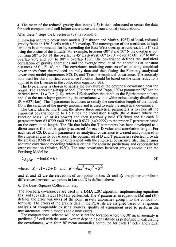
error estimation (Moritz, 1980). The auto covariance between gravity anomalies in the
Forsberg Model is:
C!::,.g!::,.g = -log(Z + R)
(4)
where: Z = zl + z2 + D and R = ~ dx 2 + dy2 + Z2
and zl and z2 are the elevations of two points in km; dx and dy are planar coordinate
differences between two points in km and D is defined above.
6. The Least-Squares Collocation Step
The Forsberg covariances are used in a DMA LSC algorithm implementing equations
(3a) and (3b) after steps (1-5) are perfonned. The V parameter in equations (3a) and (3b)
defines the error variances of the point gravity anomalies going into the collocation
fonnulre. The errors of the gravity data in the PGA file are assigned based on a rigorous
analysis of comparable existing sources, quality of equipment used to perform the
measurements, terrain models and datum errors.
The computational scheme will be to select the location where the 30' mean anomaly is
predicted (1 ° cell with the same overlap depending on latitude as perfonned in calculating
the covariances, with four 30' mean anomalies computed for each 1 ° cell). Individual
87
for each computational cell before covariance and mean anomaly calculations.
After these 4 steps the L vector in (3a) is complete.
5. Develop accurate covariance models (Heiskanen and Moritz, 1967) of local, reduced
gravity fields in 1 Ox 1 ° cells with a 30' overlap. The convergence of the meridians in high
latitudes is compensated for by extending the East-West overlap around each 1 °xl ° cell
using the cosine of the latitude. For example, between -30° S and 30° N the overlap is 30'
but from 50° to 60° N the overlap is 45' East-West; 60° to 70° - overlap 60'; 70° to 80° -
overlap 90'; and 80° to 90° - overlap 180'. The covariance defines the statistical
correlation of gravity anomalies and the average product of the anomalies at constant
distances of 0', 2', 4', etc. The covariance modeling consists of calculating empirical
covariances from the reduced anomaly data and then fitting the Forsberg analytical
covariance model parameters (CO, D, and T) to the empirical covariance. The anomaly
data used for the empirical covariance function should be based on the same reductions
applied to the L vector in the collocation equation (3a).
The D parameter is chosen to satisfy the curvature of the empirical covariance near the
origin. The Tscheming-Rapp Model (Tscheming and Rapp, 1974) parameter "s" can be
derived from D = R * (I-S) where D/2 describes the depth to the Bjerhamroar sphere,
and also the mass layer generating the covariance with a white noise density distribution
(R = 6371 km). The T parameter is chosen to satisfy the correlation length of the model.
CO is the variance of the gravity anomaly and is used to scale the analytical covariance.
The basic idea behind fitting the above three analytical parameters is to store all the
empirical covariances up to 1.5 times the correlation length (the distance where the
function loses 1/2 of its power) and then rigorously hold CO fixed and fit each D
parameter from 63.0729 (s=O.9901) to 0.6371 (s=O.9999) to the proper T parameter based
on the correlation length. The file that holds the T parameters has been developed as a
direct access file and is quickly accessed for each D value and correlation length. For
each set of CO, D, and T parameters an analytical covariance is created and compared to
the empirical gravity covariance. The optimal set of D and T parameters selected, provide
the smallest RMS of fit when differenced with the empirical covariance file. This ensures
accurate covariance modeling which is critical for accurate predictions and especially for
error estimation (Moritz, 1980). The auto covariance between gravity anomalies in the
Forsberg Model is:
C!::,.g!::,.g = -log(Z + R)
(4)
where: Z = zl + z2 + D and R = ~ dx 2 + dy2 + Z2
and zl and z2 are the elevations of two points in km; dx and dy are planar coordinate
differences between two points in km and D is defined above.
6. The Least-Squares Collocation Step
The Forsberg covariances are used in a DMA LSC algorithm implementing equations
(3a) and (3b) after steps (1-5) are perfonned. The V parameter in equations (3a) and (3b)
defines the error variances of the point gravity anomalies going into the collocation
fonnulre. The errors of the gravity data in the PGA file are assigned based on a rigorous
analysis of comparable existing sources, quality of equipment used to perform the
measurements, terrain models and datum errors.
The computational scheme will be to select the location where the 30' mean anomaly is
predicted (1 ° cell with the same overlap depending on latitude as perfonned in calculating
the covariances, with four 30' mean anomalies computed for each 1 ° cell). Individual
87