

gravity gradients
parameters.
The selected area is located in
the
Greenland-IcelandNorwegian Sea (GIN Sea) close
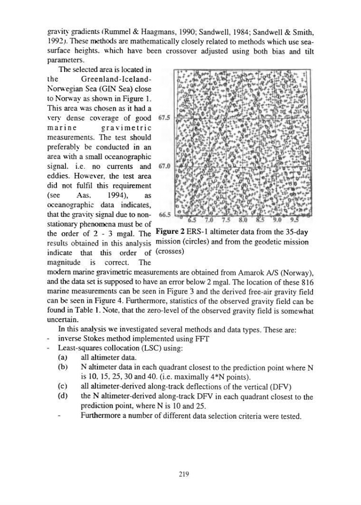
to Norway as shown in Figure L
This area was chosen as it had a
very dense covera~e of (Jood 67.5
•
_
z:::
marine
gravimetric
measurements. The test should
preferably be conducted in an
area \\1th a small oceanographic
signaL i.e. no currents and 67.0 It+1''7b.H~~,¥~J,L,;~~~t+.;*~1ri!~'tr::m
eddies. However, the test area
did not fulfil this requirement
(see
Aas.
1994),
as
oceanographic data indicates,
magnitude is correct.
modem marine gravimetric measurements are obtained from Amarok NS (Norway),
and the data set is supposed to have an error below 2 mgaL The location of these 816
marine measurements can be seen in Figure 3 and the derived free-air gravity field
can be seen in Figure 4. Furthermore, statistics of the observed gravity field can be
found in Table 1. Note, that the zero-level of the observed gravity field is somewhat
uncenain.
In this analysis we investigated several methods and data types . These are:
inverse Stokes method implemented using FFT
Least-squares collocation (LSe) using:
(a)
all altimeter data.
(b)
N altimeter data in each quadrant closest to the prediction point where N
is 10, 15, 25, 30 and 40. (i .e. maximally 4*N points).
(c)
all altimeter-derived along-track deflections of the vertical (DFV)
(d)
the N altimeter-derived along-track DFV in each quadrant closest to the
prediction point, where N is 10 and 25.
Furthermore a number of different data selection criteria were tested.
219
parameters.
The selected area is located in
the
Greenland-IcelandNorwegian Sea (GIN Sea) close
to Norway as shown in Figure L
This area was chosen as it had a
very dense covera~e of (Jood 67.5
•
_
z:::
marine
gravimetric
measurements. The test should
preferably be conducted in an
area \\1th a small oceanographic
signaL i.e. no currents and 67.0 It+1''7b.H~~,¥~J,L,;~~~t+.;*~1ri!~'tr::m
eddies. However, the test area
did not fulfil this requirement
(see
Aas.
1994),
as
oceanographic data indicates,
magnitude is correct.
modem marine gravimetric measurements are obtained from Amarok NS (Norway),
and the data set is supposed to have an error below 2 mgaL The location of these 816
marine measurements can be seen in Figure 3 and the derived free-air gravity field
can be seen in Figure 4. Furthermore, statistics of the observed gravity field can be
found in Table 1. Note, that the zero-level of the observed gravity field is somewhat
uncenain.
In this analysis we investigated several methods and data types . These are:
inverse Stokes method implemented using FFT
Least-squares collocation (LSe) using:
(a)
all altimeter data.
(b)
N altimeter data in each quadrant closest to the prediction point where N
is 10, 15, 25, 30 and 40. (i .e. maximally 4*N points).
(c)
all altimeter-derived along-track deflections of the vertical (DFV)
(d)
the N altimeter-derived along-track DFV in each quadrant closest to the
prediction point, where N is 10 and 25.
Furthermore a number of different data selection criteria were tested.
219