

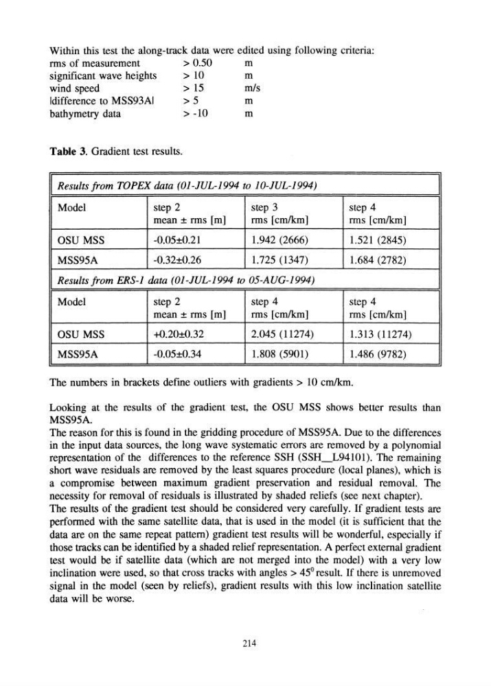
Within this test the along-track data were edited using following criteria:
nns of measurement
> 0.50
m
significant wave heights
> 1 0 m
wind speed
> 15
mls
Idifference to MSS93AI
> 5
m
bathymetry data
> -10
m
Table 3. Gradient test results.
Results from TOPEX data (Ol-JUL-1994 to lO-JUL-1994)
Model
step 2
step 3
step 4
mean ± nns [m]
nns [cmlkm]
rms [cmlkm]
OSU MSS
-0.05±0.21
1.942 (2666)
1.521 (2845)
MSS95A
-0.32±0.26
1.725 (1347)
1.684 (2782)
Results from ERS-l data (Ol-JUL-1994 to 05-AUG-1994)
Model
step 2
step 4
step 4
mean ± nns [m]
nns [cmlkm]
nns [cmlkm]
OSU MSS
+O.20±O.32
2.045 (11274)
1.313 (11274)
MSS95A
-0.05±0.34
1.808 (5901)
1.486 (9782)
The numbers in brackets defme outliers with gradients> 10 cmlkm.
Looking at the results of the gradient test, the OSU MSS shows better results than
MSS95A.
The reason for this is found in the gridding procedure of MSS95A. Due to the differences
in the input data sources, the long wave systematic errors are removed by a polynomial
representation of the differences to the reference SSH (SSH_L94101). The remaining
short wave residuals are removed by the least squares procedure (local planes), which is
a compromise between maximum gradient preservation and residual removal. The
necessity for removal of residuals is illustrated by shaded reliefs (see next chapter).
The results of the gradient test should be considered very carefully. If gradient tests are
perfonned with the same satellite data, that is used in the model (it is sufficient that the
data are on the same repeat pattern) gradient test results will be wonderful, especially if
those tracks can be identified by a shaded relief representation. A perfect external gradient
test would be if satellite data (which are not merged into the model) with a very low
inclination were used, so that cross tracks with angles > 45° result. If there is unremoved
signal in the model (seen by reliefs), gradient results with this low inclination satellite
data will be worse.
214
nns of measurement
> 0.50
m
significant wave heights
> 1 0 m
wind speed
> 15
mls
Idifference to MSS93AI
> 5
m
bathymetry data
> -10
m
Table 3. Gradient test results.
Results from TOPEX data (Ol-JUL-1994 to lO-JUL-1994)
Model
step 2
step 3
step 4
mean ± nns [m]
nns [cmlkm]
rms [cmlkm]
OSU MSS
-0.05±0.21
1.942 (2666)
1.521 (2845)
MSS95A
-0.32±0.26
1.725 (1347)
1.684 (2782)
Results from ERS-l data (Ol-JUL-1994 to 05-AUG-1994)
Model
step 2
step 4
step 4
mean ± nns [m]
nns [cmlkm]
nns [cmlkm]
OSU MSS
+O.20±O.32
2.045 (11274)
1.313 (11274)
MSS95A
-0.05±0.34
1.808 (5901)
1.486 (9782)
The numbers in brackets defme outliers with gradients> 10 cmlkm.
Looking at the results of the gradient test, the OSU MSS shows better results than
MSS95A.
The reason for this is found in the gridding procedure of MSS95A. Due to the differences
in the input data sources, the long wave systematic errors are removed by a polynomial
representation of the differences to the reference SSH (SSH_L94101). The remaining
short wave residuals are removed by the least squares procedure (local planes), which is
a compromise between maximum gradient preservation and residual removal. The
necessity for removal of residuals is illustrated by shaded reliefs (see next chapter).
The results of the gradient test should be considered very carefully. If gradient tests are
perfonned with the same satellite data, that is used in the model (it is sufficient that the
data are on the same repeat pattern) gradient test results will be wonderful, especially if
those tracks can be identified by a shaded relief representation. A perfect external gradient
test would be if satellite data (which are not merged into the model) with a very low
inclination were used, so that cross tracks with angles > 45° result. If there is unremoved
signal in the model (seen by reliefs), gradient results with this low inclination satellite
data will be worse.
214