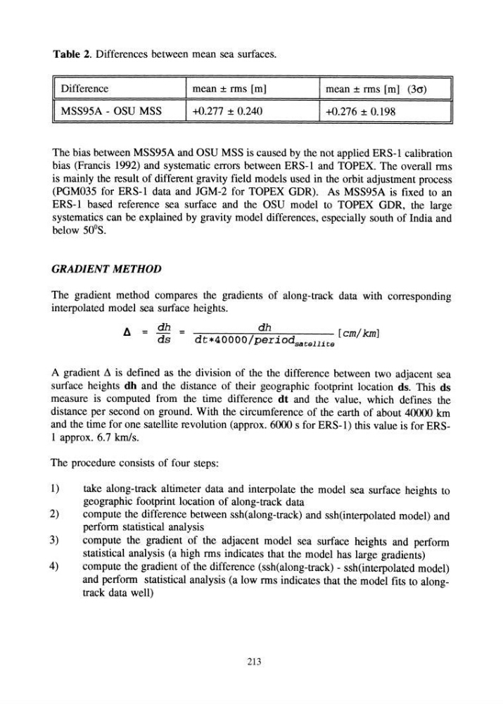
Table 2. Differences between mean sea surfaces.
I Difference
I mean ± rms [m]
I mean ± rms [m] (30')
MSS95A - OSU MSS
I +0.277 ± 0.240
I +0.276 ± 0.198
The bias between MSS95A and OSU MSS is caused by the not applied ERS-l calibration
bias (Francis 1992) and systematic errors between ERS-l and TOPEX. The overall rms
is mainly the result of different gravity field models used in the orbit adjustment process
(PGM035 for ERS-l data and JGM-2 for TOPEX GDR). As MSS95A is fixed to an
ERS-l based reference sea surface and the OSU model to TOPEX GDR, the large
systematics can be explained by gravity model differences, especially south of India and
below 50 0 S.
GRADIENT METHOD
The gradient method compares the gradients of along-track data with corresponding
interpolated model sea surface heights.
Il = db =
db .
[cm/km]
ds
dt*40000/peI~odsat;611it;6
A gradient L\ is defined as the division of the the difference between two adjacent sea
surface heights db and the distance of their geographic footprint location ds. This ds
measure is computed from the time difference dt and the value, which defines the
distance per second on ground. With the circumference of the earth of about 40000 km
and the time for one satellite revolution (approx. 6000 s for ERS-l) this value is for ERSI approx. 6.7 kmls.
The procedure consists of four steps:
1)
take along-track altimeter data and interpolate the model sea surface heights to
geographic footprint location of along-track data
2)
compute the difference between ssh(along-track) and ssh(interpolated model) and
perform statistical analysis
3)
compute the gradient of the adjacent model sea surface heights and perform
statistical analysis (a high rms indicates that the model has large gradients)
4)
compute the gradient of the difference (ssh(along-track) - ssh(interpolated model)
and perform statistical analysis (a low rms indicates that the model fits to alongtrack data well)
213