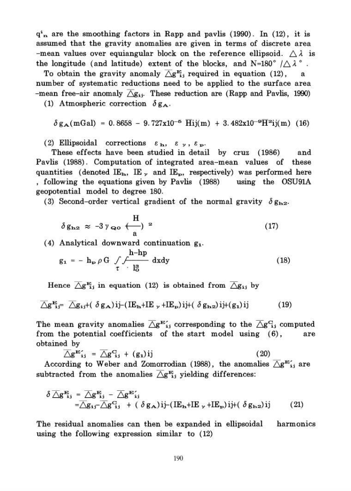
q\: .. are the smoothing factors in Rapp and pavlis (1990). In (12), it is
assumed that the gravity anomalies are given in terms of discrete area
-mean values over equiangular block on the reference ellipsoid. L.A. is
the longitude (and latitude) extent of the blocks, and N=180° /L.A. ° .
To obtain the gravity anomaly 6g~j required in equation (12),
a
number of systematic reductions need to be applied to the surface area
-mean free-air anomaly 6gij. These reduction are (Rapp and Pavlis, 1990)
(1) Atmospheric correction ~ gAo
~ gA(mGal) = 0.8658 - 9.727xl0- 5 Hij(m) + 3.482xl0- 9 H 2 ij(m) (16)
(2) Ellipsoidal corrections e h, e 'Y, e p.
These effects have been studied in detail by cruz (1986)
and
Pavlis (1988). Computation of integrated area-mean values of these
quantities (denoted IEh , IE 'Y and IEp, respectively) was performed here
, following the equations given by Pavlis (1988)
using the OSU91A
geopotential model to degree 180.
(3) Second-order vertical gradient of the normal gravity ~ gh2.
H
~ gh2 ~ -3 ' )' QO f--) 2
a
(4) Analytical downward continuation g1.
h-hp
g 1 = - hp p G .f .f
dxdy
't' . m
Hence 6g~j in equation (12) is obtained from 6gij by
(17)
(18)
The mean gravity anomalies 6gE~j corresponding to the 6g~j computed
from the potential coefficients of the start model using (6) ,
are
obtained by
6gE~j = 6g~j + (g1) ij
(20)
According to Weber and Zomorrodian (1988), the anomalies 6gE~j are
subtracted from the anomalies 6g~j yielding differences:
~ 6g~j = 6g~j _ 6gE~j
= 6gir 6g~j + ( ~ gA) ij-( IEh + IE 'Y + IEp) ij+( ~ gh2) ij
(21)
The residual anomalies can then be expanded in ellipsoidal
harmonics
using the following expression similar to (12)
190