

effective estimates since variations in the higher degree zonals can not be independently
estimated.
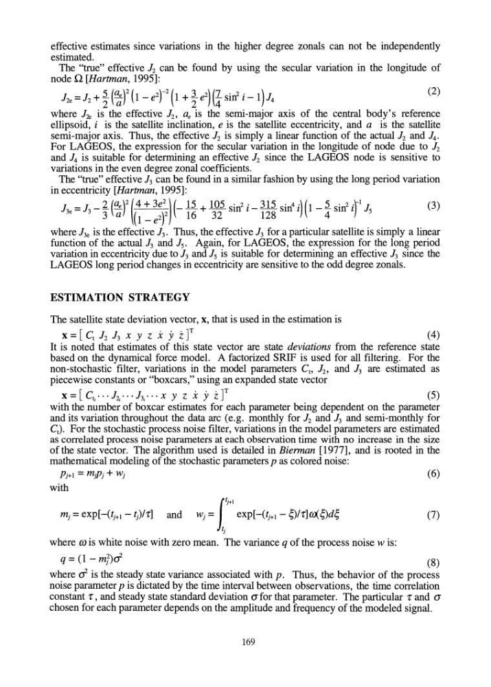
The "true" effective 12 can be found by using the secular variation in the longitude of
node n [Hartman, 1995]:
12e=12+r(~y(I -e 2 t(1 +te2)(~sin2 i-l)14
(2)
where 12e is the effective 1 2 , a e is the semi-major axis of the central body's reference
ellipsoid, i is the satellite inclination, e is the satellite eccentricity, and a is the satellite
semi-major axis. Thus, the effective 12 is simply a linear function of the actual 12 and 14.
For LAGEOS, the expression for the secular variation in the longitude of node due to 12
and 14 is suitable for determining an effective 12 since the LAGEOS node is sensitive to
variations in the even degree zonal coefficients.
The "true" effective 13 can be found in a similar fashion by using the long period variation
in eccentricity [Hartman, 1995]:
J =J _2.(a e )2(4+3e 2 )(_ll+ 105 sin 2 i_ 315 sin4i)(I- i sin2ifl J
3e
3
3 a (
)2
16 32
128
4
) 5
1- e 2
(3)
where 13e is the effective 1 3 . Thus, the effective 13 for a particular satellite is simply a linear
function of the actual 13 and 1 5 . Again, for LAGEOS, the expression for the long period
variation in eccentricity due to 13 and 15 is suitable for determining an effective 13 since the
LAGEOS long period changes in eccentricity are sensitive to the odd degree zonals.
ESTIMATION STRATEGY
The satellite state deviation vector, x, that is used in the estimation is
x = [ Ct 12 13 X Y z X Y zJT
(4)
It is noted that estimates of this state vector are state deviations from the reference state
based on the dynamical force model. A factorized SRIF is used for all filtering. For the
non-stochastic filter, variations in the model parameters C t , 1 2 , and 13 are estimated as
piecewise constants or "boxcars," using an expanded state vector
x = [ C t ;· •• 12; ... 1 3 ; .•• x y z X y Z Y
(5)
with the number of boxcar estimates for each parameter being dependent on the parameter
and its variation throughout the data arc (e.g. monthly for 12 and 13 and semi-monthly for
C t ). For the stochastic process noise filter, variations in the model parameters are estimated
as correlated process noise parameters at each observation time with no increase in the size
of the state vector. The algorithm used is detailed in Bierman [1977], and is rooted in the
mathematical modeling of the stochastic parameters P as colored noise:
PM = mjpj + Wj
with
mj = exp[-(tj+1 - t)/-r] and Wj = 1"" expHtj>l- ~/~lOX~~
J
where m is white noise with zero mean. The variance q of the process noise W is:
(6)
(7)
q = (l - mJ)cf
(8)
where d is the steady state variance associated with p. Thus, the behavior of the process
noise parameter p is dictated by the time interval between observations, the time correlation
constant -r, and steady state standard deviation a for that parameter. The particular -r and a
chosen for each parameter depends on the amplitude and frequency of the modeled signal.
169
estimated.
The "true" effective 12 can be found by using the secular variation in the longitude of
node n [Hartman, 1995]:
12e=12+r(~y(I -e 2 t(1 +te2)(~sin2 i-l)14
(2)
where 12e is the effective 1 2 , a e is the semi-major axis of the central body's reference
ellipsoid, i is the satellite inclination, e is the satellite eccentricity, and a is the satellite
semi-major axis. Thus, the effective 12 is simply a linear function of the actual 12 and 14.
For LAGEOS, the expression for the secular variation in the longitude of node due to 12
and 14 is suitable for determining an effective 12 since the LAGEOS node is sensitive to
variations in the even degree zonal coefficients.
The "true" effective 13 can be found in a similar fashion by using the long period variation
in eccentricity [Hartman, 1995]:
J =J _2.(a e )2(4+3e 2 )(_ll+ 105 sin 2 i_ 315 sin4i)(I- i sin2ifl J
3e
3
3 a (
)2
16 32
128
4
) 5
1- e 2
(3)
where 13e is the effective 1 3 . Thus, the effective 13 for a particular satellite is simply a linear
function of the actual 13 and 1 5 . Again, for LAGEOS, the expression for the long period
variation in eccentricity due to 13 and 15 is suitable for determining an effective 13 since the
LAGEOS long period changes in eccentricity are sensitive to the odd degree zonals.
ESTIMATION STRATEGY
The satellite state deviation vector, x, that is used in the estimation is
x = [ Ct 12 13 X Y z X Y zJT
(4)
It is noted that estimates of this state vector are state deviations from the reference state
based on the dynamical force model. A factorized SRIF is used for all filtering. For the
non-stochastic filter, variations in the model parameters C t , 1 2 , and 13 are estimated as
piecewise constants or "boxcars," using an expanded state vector
x = [ C t ;· •• 12; ... 1 3 ; .•• x y z X y Z Y
(5)
with the number of boxcar estimates for each parameter being dependent on the parameter
and its variation throughout the data arc (e.g. monthly for 12 and 13 and semi-monthly for
C t ). For the stochastic process noise filter, variations in the model parameters are estimated
as correlated process noise parameters at each observation time with no increase in the size
of the state vector. The algorithm used is detailed in Bierman [1977], and is rooted in the
mathematical modeling of the stochastic parameters P as colored noise:
PM = mjpj + Wj
with
mj = exp[-(tj+1 - t)/-r] and Wj = 1"" expHtj>l- ~/~lOX~~
J
where m is white noise with zero mean. The variance q of the process noise W is:
(6)
(7)
q = (l - mJ)cf
(8)
where d is the steady state variance associated with p. Thus, the behavior of the process
noise parameter p is dictated by the time interval between observations, the time correlation
constant -r, and steady state standard deviation a for that parameter. The particular -r and a
chosen for each parameter depends on the amplitude and frequency of the modeled signal.
169