

FILTERING RESULTS
The simulated one year data arc with model deviation signals present for C t , 1 2 , 1 3 , 1 4 , and
15 is processed. A single estimate is made for the satellite state, and no estimate is made for
14 or 1 5 , even though 14 and 15 model deviation signals are present in the data. This
configuration assesses the ability of each filter to resolve the C t variation and the effective 12
and 13 temporal variations.
The standard SRIF is implemented using 24 consecutive 15 day estimates for C t and 12
consecutive one month estimates for 12 and 13 throughout the arc. The process noise SRIF
is implemented with stochastic estimates made for C t , 1 2 , and 1 3 , Stochastic estimates of
each parameter, based on specific values of 7: and a, are made at every time that an
observation exists. The values of 7: and a used for each parameter in the stochastic fIlter
are shown in Table 1.
The non-stochastic and stochastic estimates for the C t , 1 2 , and 13 temporal variations are
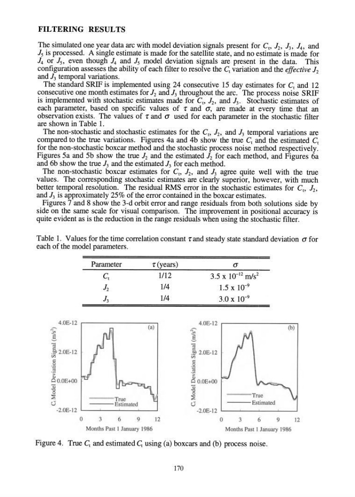
compared to the true variations. Figures 4a and 4b show the true C t and the estimated C t
for the non-stochastic boxcar method and the stochastic process noise method respectively.
Figures 5a and 5b show the true 12 and the estimated 12 for each method, and Figures 6a
and 6b show the true 13 and the estimated 13 for each method.
The non-stochastic boxcar estimates for C t , 1 2 , and 13 agree quite well with the true
values. The corresponding stochastic estimates are clearly superior, however, with much
better temporal resolution. The residual RMS error in the stochastic estimates for C t , 1 2 ,
and 13 is approximately 25% of the error contained in the boxcar estimates.
Figures 7 and 8 show the 3-d orbit error and range residuals from both solutions side by
side on the same scale for visual comparison. The improvement in positional accuracy is
quite evident as is the reduction in the range residuals when using the stochastic fIlter.
Table 1. Values for the time correlation constant 7: and steady state standard deviation a for
each of the model parameters.
Parameter
7: (years)
C t
12
13
--i
4.0E-12 .--------~
(a)
«i
c
.!:.O 2.0E-12
en
c
o
'0
'"
't
QO.OE+OO
<3
-g
~
o
- - -True
- - - E limated
-2.0E-12 '--_....!.-_--'-_---1_----'
1112
1/4
114
o
3
6
9
12
Month Past 1 January 1986
a
3.5 x 10- 12 rnls 2
1.5 x 10- 9
3.0 x 10- 9
~
4.0E-12 r - - - - - - - - ( b = - : ) - ,
'-'
«i
.~ 2.0E-12
en
c
o
'0
t'd
.;;;
o
Q O. OE+OO
Q)
-g
~
o
- - -True
---Estimated
-2.0E-12 ' - - - - - -- - - - - - '
o
3
6
9
12
Months Past I January 1986
Figure 4. True C t and estimated G using (a) boxcars and (b) process noise.
170
The simulated one year data arc with model deviation signals present for C t , 1 2 , 1 3 , 1 4 , and
15 is processed. A single estimate is made for the satellite state, and no estimate is made for
14 or 1 5 , even though 14 and 15 model deviation signals are present in the data. This
configuration assesses the ability of each filter to resolve the C t variation and the effective 12
and 13 temporal variations.
The standard SRIF is implemented using 24 consecutive 15 day estimates for C t and 12
consecutive one month estimates for 12 and 13 throughout the arc. The process noise SRIF
is implemented with stochastic estimates made for C t , 1 2 , and 1 3 , Stochastic estimates of
each parameter, based on specific values of 7: and a, are made at every time that an
observation exists. The values of 7: and a used for each parameter in the stochastic fIlter
are shown in Table 1.
The non-stochastic and stochastic estimates for the C t , 1 2 , and 13 temporal variations are
compared to the true variations. Figures 4a and 4b show the true C t and the estimated C t
for the non-stochastic boxcar method and the stochastic process noise method respectively.
Figures 5a and 5b show the true 12 and the estimated 12 for each method, and Figures 6a
and 6b show the true 13 and the estimated 13 for each method.
The non-stochastic boxcar estimates for C t , 1 2 , and 13 agree quite well with the true
values. The corresponding stochastic estimates are clearly superior, however, with much
better temporal resolution. The residual RMS error in the stochastic estimates for C t , 1 2 ,
and 13 is approximately 25% of the error contained in the boxcar estimates.
Figures 7 and 8 show the 3-d orbit error and range residuals from both solutions side by
side on the same scale for visual comparison. The improvement in positional accuracy is
quite evident as is the reduction in the range residuals when using the stochastic fIlter.
Table 1. Values for the time correlation constant 7: and steady state standard deviation a for
each of the model parameters.
Parameter
7: (years)
C t
12
13
--i
4.0E-12 .--------~
(a)
«i
c
.!:.O 2.0E-12
en
c
o
'0
'"
't
QO.OE+OO
<3
-g
~
o
- - -True
- - - E limated
-2.0E-12 '--_....!.-_--'-_---1_----'
1112
1/4
114
o
3
6
9
12
Month Past 1 January 1986
a
3.5 x 10- 12 rnls 2
1.5 x 10- 9
3.0 x 10- 9
~
4.0E-12 r - - - - - - - - ( b = - : ) - ,
'-'
«i
.~ 2.0E-12
en
c
o
'0
t'd
.;;;
o
Q O. OE+OO
Q)
-g
~
o
- - -True
---Estimated
-2.0E-12 ' - - - - - -- - - - - - '
o
3
6
9
12
Months Past I January 1986
Figure 4. True C t and estimated G using (a) boxcars and (b) process noise.
170