

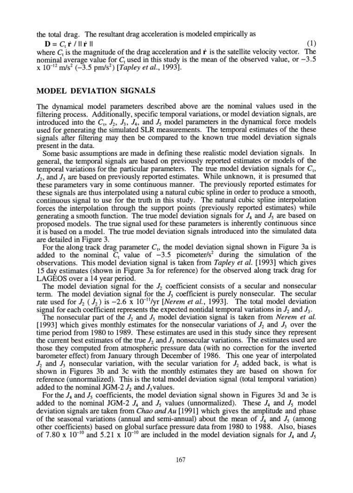
the total drag. The resultant drag acceleration is modeled empirically as
D ::;: C t rill r II
(l)
where C t is the magnitude of the drag acceleration and r is the satellite velocity vector. The
nominal average value for C t used in this study is the mean of the observed value, or -3.5
x 10- 12 m/s 2 (-3.5 pm/s 2 ) [Tapley et ai., 1993].
MODEL DEVIATION SIGNALS
The dynamical model parameters described above are the nominal values used in the
filtering process. Additionally, specific temporal variations, or model deviation signals, are
introduced into the C t , 1 2 , 1 3 , 1 4 , and 15 model parameters in the dynamical force models
used for generating the simulated SLR measurements. The temporal estimates of the these
signals after fIltering may then be compared to the known true model deviation signals
present in the data.
Some basic assumptions are made in defining these realistic model deviation signals. In
general, the temporal signals are based on previously reported estimates or models of the
temporal variations for the particular parameters. The true model deviation signals for Ct,
1 2 , and 13 are based on previously reported estimates. While unknown, it is presumed that
these parameters vary in some continuous manner. The previously reported estimates for
these signals are thus interpolated using a natural cubic spline in order to produce a smooth,
continuous signal to use for the truth in this study. The natural cubic spline interpolation
forces the interpolation through the support points (previously reported estimates) while
generating a smooth function. The true model deviation signals for 14 and 15 are based on
proposed models. The true signal used for these parameters is inherently continuous since
it is based on a model. The true model deviation signals introduced into the simulated data
are detailed in Figure 3.
For the along track drag parameter Ct, the model deviation signal shown in Figure 3a is
added to the nominal C t value of -3.5 picometerls 2 during the simulation of the
observations. This model deviation signal is taken from Tapley et al. [1993] which gives
15 day estimates (shown in Figure 3a for reference) for the observed along track drag for
LAGEOS over a 14 year period.
The model deviation signal for the 12 coefficient consists of a secular and nonsecular
term. The model ~eviation signal for the 13 coefficient is purely nonsecular. The secular
rate used for 12 (1 2 ) is -2.6 x 1O- 11 /yr [Nerem et aI., 1993]. The total model deviation
signal for each coefficient represents the expected nontidal temporal variations in J 2 and 1 3 ,
The nonsecular part of the 12 and 13 model deviation signal is taken from Nerem et al.
[1993] which gives monthly estimates for the nonsecular variations of 12 and 13 over the
time period from 1980 to 1989. These estimates are used in this study since they represent
the current best estimates of the true 12 and 13 nonsecular variations. The estimates used are
those they computed from atmospheric pressure data (with no correction for the inverted
barometer effect) from January through December of 1986. This one year of interpolated
12 and 13 nonsecular variation, with the secular variation for 12 added back, is what is
shown in Figures 3b and 3c with the monthly estimates they are based on shown for
reference (unnormalized). This is the total model deviation signal (total temporal variation)
added to the nominal JGM-2 12 and 13 values.
For the 14 and 15 coefficients, the model deviation signal shown in Figures 3d and 3e is
added to the nominal JGM-2 14 and 15 values (unnormalized). These 14 and 15 model
deviation signals are taken from Chao andAu [1991] which gives the amplitude and phase
of the seasonal variations (annual and semi-annual) about the mean of 14 and 15 (among
other coefficients) based on global surface pressure data from 1980 to 1988. Also, biases
of 7.80 x 10- 10 and 5.21 x 10- 10 are included in the model deviation signals for 14 and 15
167
D ::;: C t rill r II
(l)
where C t is the magnitude of the drag acceleration and r is the satellite velocity vector. The
nominal average value for C t used in this study is the mean of the observed value, or -3.5
x 10- 12 m/s 2 (-3.5 pm/s 2 ) [Tapley et ai., 1993].
MODEL DEVIATION SIGNALS
The dynamical model parameters described above are the nominal values used in the
filtering process. Additionally, specific temporal variations, or model deviation signals, are
introduced into the C t , 1 2 , 1 3 , 1 4 , and 15 model parameters in the dynamical force models
used for generating the simulated SLR measurements. The temporal estimates of the these
signals after fIltering may then be compared to the known true model deviation signals
present in the data.
Some basic assumptions are made in defining these realistic model deviation signals. In
general, the temporal signals are based on previously reported estimates or models of the
temporal variations for the particular parameters. The true model deviation signals for Ct,
1 2 , and 13 are based on previously reported estimates. While unknown, it is presumed that
these parameters vary in some continuous manner. The previously reported estimates for
these signals are thus interpolated using a natural cubic spline in order to produce a smooth,
continuous signal to use for the truth in this study. The natural cubic spline interpolation
forces the interpolation through the support points (previously reported estimates) while
generating a smooth function. The true model deviation signals for 14 and 15 are based on
proposed models. The true signal used for these parameters is inherently continuous since
it is based on a model. The true model deviation signals introduced into the simulated data
are detailed in Figure 3.
For the along track drag parameter Ct, the model deviation signal shown in Figure 3a is
added to the nominal C t value of -3.5 picometerls 2 during the simulation of the
observations. This model deviation signal is taken from Tapley et al. [1993] which gives
15 day estimates (shown in Figure 3a for reference) for the observed along track drag for
LAGEOS over a 14 year period.
The model deviation signal for the 12 coefficient consists of a secular and nonsecular
term. The model ~eviation signal for the 13 coefficient is purely nonsecular. The secular
rate used for 12 (1 2 ) is -2.6 x 1O- 11 /yr [Nerem et aI., 1993]. The total model deviation
signal for each coefficient represents the expected nontidal temporal variations in J 2 and 1 3 ,
The nonsecular part of the 12 and 13 model deviation signal is taken from Nerem et al.
[1993] which gives monthly estimates for the nonsecular variations of 12 and 13 over the
time period from 1980 to 1989. These estimates are used in this study since they represent
the current best estimates of the true 12 and 13 nonsecular variations. The estimates used are
those they computed from atmospheric pressure data (with no correction for the inverted
barometer effect) from January through December of 1986. This one year of interpolated
12 and 13 nonsecular variation, with the secular variation for 12 added back, is what is
shown in Figures 3b and 3c with the monthly estimates they are based on shown for
reference (unnormalized). This is the total model deviation signal (total temporal variation)
added to the nominal JGM-2 12 and 13 values.
For the 14 and 15 coefficients, the model deviation signal shown in Figures 3d and 3e is
added to the nominal JGM-2 14 and 15 values (unnormalized). These 14 and 15 model
deviation signals are taken from Chao andAu [1991] which gives the amplitude and phase
of the seasonal variations (annual and semi-annual) about the mean of 14 and 15 (among
other coefficients) based on global surface pressure data from 1980 to 1988. Also, biases
of 7.80 x 10- 10 and 5.21 x 10- 10 are included in the model deviation signals for 14 and 15
167