

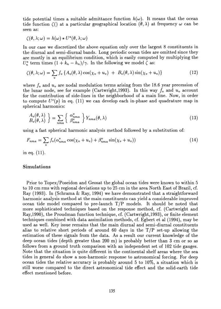
tide potential times a suitable admittance function h(w). It means that the ocean
tide function (0 at a particular geographical location (0, A) at frequency w can be
seen as:
In our case we discretized the above equation only over the largest 8 constituents in
the diurnal and semi-diurnal bands. Long periodic ocean tides are omitted since they
are mostly in an equilibrium condition, which is easily computed by multiplying the
U~ term times (1 + kn - hn )/,. In the following we model ( as:
(12)
v
where Iv and U v are nodal modulation terms arising from the 18.6 year precession of
the lunar node, see for example (Cartwright,1993). In this way Iv and U v account
for the contribution of side-lines in the neighborhood of a main line. Now, in order
to compute UO(p) in eq. (11) we can develop each in-phase and quadrature map in
spherical harmonics:
Av(O, A)} " { a~ma } y. (II ')
B (0 A) = L...t Qv
nma rJ, A
v,
nma fJnma
(13)
using a fast spherical harmonic analysis method followed by a substitution of:
Fnma = I: Iv(a~ma cos(xv + uv) + f3:ma sin(xv + uv))
(14)
v
in eq. (11).
Simulations
Prior to Topex/Poseidon and Geosat the global ocean tides were known to within 5
to 10 cm rms with regional deviations up to 25 cm in the area North E~st of Brazil, cf.
Ray (1993). In (Schrama & Ray, 1994) we have demonstrated that a straightforward
harmonic analysis method at the main constituents can yield a considerable improved
ocean tide model compared to pre-launch T/P models. It should be noted that
more sophisticated techniques based on the response method, cf. (Cartwright and
Ray,1990), the Proudman function technique, cf. (Cartwright,1993), or finite element
techniques combined with data assimilation methods, cf. Egbert et al (1994), may be
used as well. Key issue remains that the main diurnal and semi-diurnal constituents
alias to relative short periods of around 60 days in the T /P set-up allowing the
estimation of these signals from the data. As a result our current knowledge of the
deep ocean tides (depth greater than 200 m) is probably better than 3 cm or so as
follows from a ground truth comparison with an independent set of 102 tide gauges.
Note that the situation is quite different in the continental shelf areas where the sea
tides in general do show a non-harmonic response to astronomical forcing. For deep
ocean tides the relative accuracy is probably around 5 to 10%, a situation which is
still worse compared to the direct astronomical tide effect and the solid-earth tide
effect mentioned before.
135
tide function (0 at a particular geographical location (0, A) at frequency w can be
seen as:
In our case we discretized the above equation only over the largest 8 constituents in
the diurnal and semi-diurnal bands. Long periodic ocean tides are omitted since they
are mostly in an equilibrium condition, which is easily computed by multiplying the
U~ term times (1 + kn - hn )/,. In the following we model ( as:
(12)
v
where Iv and U v are nodal modulation terms arising from the 18.6 year precession of
the lunar node, see for example (Cartwright,1993). In this way Iv and U v account
for the contribution of side-lines in the neighborhood of a main line. Now, in order
to compute UO(p) in eq. (11) we can develop each in-phase and quadrature map in
spherical harmonics:
Av(O, A)} " { a~ma } y. (II ')
B (0 A) = L...t Qv
nma rJ, A
v,
nma fJnma
(13)
using a fast spherical harmonic analysis method followed by a substitution of:
Fnma = I: Iv(a~ma cos(xv + uv) + f3:ma sin(xv + uv))
(14)
v
in eq. (11).
Simulations
Prior to Topex/Poseidon and Geosat the global ocean tides were known to within 5
to 10 cm rms with regional deviations up to 25 cm in the area North E~st of Brazil, cf.
Ray (1993). In (Schrama & Ray, 1994) we have demonstrated that a straightforward
harmonic analysis method at the main constituents can yield a considerable improved
ocean tide model compared to pre-launch T/P models. It should be noted that
more sophisticated techniques based on the response method, cf. (Cartwright and
Ray,1990), the Proudman function technique, cf. (Cartwright,1993), or finite element
techniques combined with data assimilation methods, cf. Egbert et al (1994), may be
used as well. Key issue remains that the main diurnal and semi-diurnal constituents
alias to relative short periods of around 60 days in the T /P set-up allowing the
estimation of these signals from the data. As a result our current knowledge of the
deep ocean tides (depth greater than 200 m) is probably better than 3 cm or so as
follows from a ground truth comparison with an independent set of 102 tide gauges.
Note that the situation is quite different in the continental shelf areas where the sea
tides in general do show a non-harmonic response to astronomical forcing. For deep
ocean tides the relative accuracy is probably around 5 to 10%, a situation which is
still worse compared to the direct astronomical tide effect and the solid-earth tide
effect mentioned before.
135