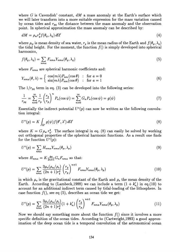
where G is Cavendish' constant, dM a mass anomaly at the Earth's surface which
we will later transform into a more suitable expression for the mass variation caused
by ocean tides and rpq the distance between the mass anomaly and the observation
point. In spherical approximation the mass anomaly can be described by:
(4)
where pw is mean density of sea water, rq is the mean radius ofthe Earth and I(Oq, Aq)
the tidal height. For the moment, the function 10 is simply developed into spherical
harmonics,
(5)
nma
where Fnma are spherical harmonic coefficients and:
y. (0 A) _ {Cos(mA)Pnm(COSO) : for a = 0
nma , -
sin(mA)Pnm(cos 0) : for a = 1
(6)
The l/rpq term in eq. (3) can be developed into the following series:
(7)
Essentially the indirect potential UO(p) can now be written as the following convolution integral:
UO(p) = K [ g(tfJ)/(O',A')dn'
in'
(8)
where K = G pw r;. The surface integral in eq. (8) can easily be solved by working
out orthogonal properties of the spherical harmonic functions. As a result one finds
for the function UO(p):
UO(p) = L HnmaYnma(Op, Ap)
(9)
nma
where Hnma = K 2!~1 GnFnma so that:
U O() ,,3J.Le(Pw/ Pe) (rq)n+l F. y. (0 \)
P = L.J (2 + 1) 2 -
nma nma p, Ap
nma n
rq rp
(10)
in which J.Le is the gravitational constant of the Earth and Pe the mean density of the
Earth. According to (Lambeck,1988) we can include a term (1 + k~) in eq.(10) to
account for an additional indirect term caused by tidal-loading of the lithosphere. In
case function 10, see eq (5), describes an ocean tide we get:
U
O ( )
,,3J.Le(Pw/Pe)(1 k') (rq)n+l F. y. (0 \)
P = L.J (2 + 1) 2 + n -
nma nma p, Ap
nma n
rq
rp
(11)
Now we should say somethiug more about the function 10 since it involves a more
specific definition of the ocean tides. According to (Cartwright,199:J) a good approximation of the deep ocean tide is a temporal convolution of the astronomical ocean
134