

include the data over the young ocean floor, the linear
scale is too small to differentiate between the models at
older ages. To enlarge the scale for the older ages, but still
retain the young data, he plotted the data with the distance
on the vertical axis scaled as 1/heat flow
2 (Figure 5b). In
such a plot, only the models of Crosby and McKenzie
(2009) and Goutorbe and Hillier (2013) give a good match
to his statistical best fit to the filtered heat flow data. However, the model of Goutorbe and Hillier (2013) has a
higher basal temperature of 1,390
and a greater plate
thickness (106–110 km). Both models match the heat flow
relation without adding the effect of crustal radioactivity.
The best-fitting heat flow age model by Hasterok
(2013), which fits the heat flow data, can be parameterized
by the following simple relationship:
For t 17.4 Ma, q ¼ 506.7 t
À1/2 .
For t > 17.4 Ma, q ¼ 53 + 106 e
À0.034607t
.
As a result of the reduction in the scatter in heat flow, it
is necessary to reconsider the variation in the topography.
It is created both by mantle plumes and their topographic
expression (Goutorbe and Hiller, 2013) (Figure 6a). In
addition, Crosby et al. (2006) have suggested that cells
small-scale convection that give rise to dynamic topography also have an effect. To investigate the importance of
this, they removed the effects of both mantle plumes and
the dynamic topography, both positive and negative, by
only considering depths in areas of low free-air gravity.
Using these data Crosby and McKenzie (2009) found that
the depth-age data in the North Pacific best fit a plate
~90 km thick and 1,315
C bottom temperature.
This plate is much thinner than the thickness of 125 km
given by Parsons and Sclater (1977). The thermal model
of Crosby and McKenzie (2009) constructed to fit the
depth-age relation also accounts for the heat flow relation
for the old ocean floor, thus allowing a single thermal
model to match both the heat flow and the depth without
assuming significant radioactivity in the ocean crust.
Crosby et al. (2006), Crosby and McKenzie (2009), and
Goutorbe and Hillier (2013) start with the assumptions of
Parsons and McKenzie (1978) where the cooling oceanic
lithosphere consists of a mechanical and thermal boundary
layer. At older ages the thermal boundary layer becomes
unstable and heat is added to the bottom of the plate
(Figure 6a). McKenzie et al. (2005) have pointed out that
the creation of a plate of constant thickness is a good
approximation to this concept. The bottom of the plate lies
within the thermal boundary layer (Figure 6b).
Both the models of Crosby and McKenzie (2009) and
Goutorbe and Hillier (2013) consider the effect of
dynamic topography within the mantle (Figure 6a). In
the case of Goutorbe and Hillier (2013), they remove only
the major plumes and their topographic expression.
Crosby and McKenzie (2009) assume that all areas where
the gravity anomaly is large are associated with smallscale dynamic topography and remove them from their
analysis. The model of Crosby and McKenzie (2009) has
the advantage of having the lower bottom temperature
for the plate fixed at ~1,315
C, and McKenzie et al. (2005)
have argued that this is the required temperature for
upwelling to make a crustal thickness of 7 km. However,
it has the disadvantage that it is statistical in basis and
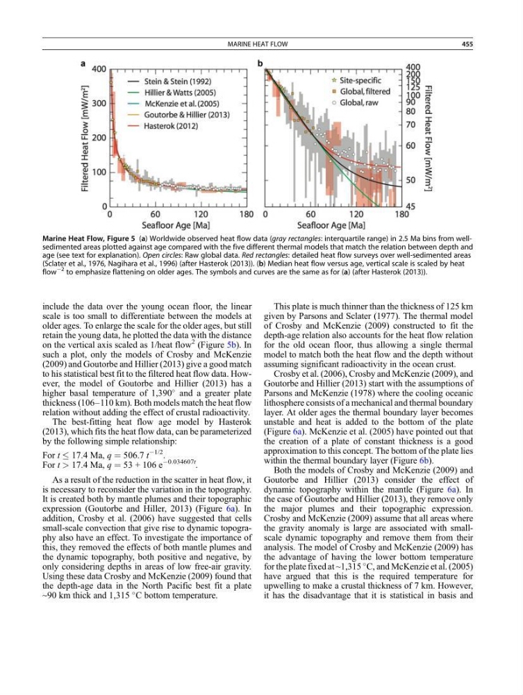
Marine Heat Flow, Figure 5 (a) Worldwide observed heat flow data (gray rectangles: interquartile range) in 2.5 Ma bins from wellsedimented areas plotted against age compared with the five different thermal models that match the relation between depth and
age (see text for explanation). Open circles: Raw global data. Red rectangles: detailed heat flow surveys over well-sedimented areas
(Sclater et al., 1976, Nagihara et al., 1996) (after Hasterok (2013)). (b) Median heat flow versus age, vertical scale is scaled by heat
flow
À2 to emphasize flattening on older ages. The symbols and curves are the same as for (a) (after Hasterok (2013)).
MARINE HEAT FLOW
455
scale is too small to differentiate between the models at
older ages. To enlarge the scale for the older ages, but still
retain the young data, he plotted the data with the distance
on the vertical axis scaled as 1/heat flow
2 (Figure 5b). In
such a plot, only the models of Crosby and McKenzie
(2009) and Goutorbe and Hillier (2013) give a good match
to his statistical best fit to the filtered heat flow data. However, the model of Goutorbe and Hillier (2013) has a
higher basal temperature of 1,390
and a greater plate
thickness (106–110 km). Both models match the heat flow
relation without adding the effect of crustal radioactivity.
The best-fitting heat flow age model by Hasterok
(2013), which fits the heat flow data, can be parameterized
by the following simple relationship:
For t 17.4 Ma, q ¼ 506.7 t
À1/2 .
For t > 17.4 Ma, q ¼ 53 + 106 e
À0.034607t
.
As a result of the reduction in the scatter in heat flow, it
is necessary to reconsider the variation in the topography.
It is created both by mantle plumes and their topographic
expression (Goutorbe and Hiller, 2013) (Figure 6a). In
addition, Crosby et al. (2006) have suggested that cells
small-scale convection that give rise to dynamic topography also have an effect. To investigate the importance of
this, they removed the effects of both mantle plumes and
the dynamic topography, both positive and negative, by
only considering depths in areas of low free-air gravity.
Using these data Crosby and McKenzie (2009) found that
the depth-age data in the North Pacific best fit a plate
~90 km thick and 1,315
C bottom temperature.
This plate is much thinner than the thickness of 125 km
given by Parsons and Sclater (1977). The thermal model
of Crosby and McKenzie (2009) constructed to fit the
depth-age relation also accounts for the heat flow relation
for the old ocean floor, thus allowing a single thermal
model to match both the heat flow and the depth without
assuming significant radioactivity in the ocean crust.
Crosby et al. (2006), Crosby and McKenzie (2009), and
Goutorbe and Hillier (2013) start with the assumptions of
Parsons and McKenzie (1978) where the cooling oceanic
lithosphere consists of a mechanical and thermal boundary
layer. At older ages the thermal boundary layer becomes
unstable and heat is added to the bottom of the plate
(Figure 6a). McKenzie et al. (2005) have pointed out that
the creation of a plate of constant thickness is a good
approximation to this concept. The bottom of the plate lies
within the thermal boundary layer (Figure 6b).
Both the models of Crosby and McKenzie (2009) and
Goutorbe and Hillier (2013) consider the effect of
dynamic topography within the mantle (Figure 6a). In
the case of Goutorbe and Hillier (2013), they remove only
the major plumes and their topographic expression.
Crosby and McKenzie (2009) assume that all areas where
the gravity anomaly is large are associated with smallscale dynamic topography and remove them from their
analysis. The model of Crosby and McKenzie (2009) has
the advantage of having the lower bottom temperature
for the plate fixed at ~1,315
C, and McKenzie et al. (2005)
have argued that this is the required temperature for
upwelling to make a crustal thickness of 7 km. However,
it has the disadvantage that it is statistical in basis and
Marine Heat Flow, Figure 5 (a) Worldwide observed heat flow data (gray rectangles: interquartile range) in 2.5 Ma bins from wellsedimented areas plotted against age compared with the five different thermal models that match the relation between depth and
age (see text for explanation). Open circles: Raw global data. Red rectangles: detailed heat flow surveys over well-sedimented areas
(Sclater et al., 1976, Nagihara et al., 1996) (after Hasterok (2013)). (b) Median heat flow versus age, vertical scale is scaled by heat
flow
À2 to emphasize flattening on older ages. The symbols and curves are the same as for (a) (after Hasterok (2013)).
MARINE HEAT FLOW
455