

the near-bottom flow at the flood tide, the vertical velocity
profile is much more uniform at the flood than at the ebb
tide. As a consequence, velocity profiles are bottom intensified during flood and surface intensified during ebb
(Burchard and Baumert, 1998). Burchand and Hetland
(2010) revealed that tidal straining is the governing process in generating estuarine circulation for periodically
stratified estuaries. The process may not only be driven
by tidal asymmetries resulting from horizontal buoyancy
gradients but from other asymmetric process as well
(e.g., wind straining). Tidal straining is the main mechanism for generation of estuarine turbidity maxima.
Spring-neap modulation of tidal forcing has been found
in many estuaries. In these estuaries during neap tides,
potential energy input due to straining by the mean gravitational circulation exceeds the buoyancy flux due to tidal
mixing and results in increase in stratification (Geyer and
MacCready, 2014).
Lateral flows in estuaries are usually much smaller than
the dominant tidal currents directed along the channel
(Lerczak and Geyer, 2004). In many systems differential
advection drives secondary flows, with the exception in
the vicinity of channel beds where flow curvature is the
main factor (Chant, 2010). The Coriolis acceleration is
the next important forcing variable influencing the estuarine secondary circulation. Lerczak and Geyer (2004)
found that the lateral flow tends to be stronger during
flood than ebb tides. Moreover, Scully et al. (2009) demonstrated that tidal rectification of lateral advection may
act as a driving force for the residual estuarine circulation.
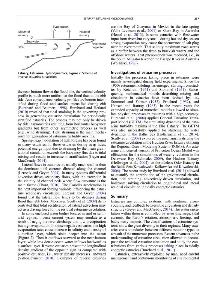
In some enclosed water bodies located in arid or semiarid regions, inverse current system may emulate as a
result of negligible river discharge and low precipitation
but high evaporation. In those negative estuaries, the high
evaporation rates cause increase in salinity and density of
a surface layer, which sinks deeper into the ocean
(Figure 2). Then it outflows seaward at the near-bottom
layer, while less dense ocean water inflows landward as
a surface layer. Reverse estuaries present the longitudinal
density gradient of the opposite sign as compared with
positive estuaries, i.e., water density increases landward
(Valle-Levinson, 2010). Examples of reverse estuaries
are the Bay of Guaymas in Mexico in the late spring
(Valle-Levinson et al., 2001) or Shark Bay in Australia
(Hetzel et al., 2013). In some estuaries with freshwater
input from rivers but very small, during hot and dry season
strong evaporation may cause the occurrence of salt plug
near the river mouth. That salinity maximum zone serves
as a buffer between the fresh to brackish waters and the
offshore waters. That phenomenon was recorded, i.e., in
the South Alligator River or the Escape River in Australia
(Wolanski, 1986).
Investigations of estuarine processes
Initially the processes taking place in estuaries were
mainly investigated during field experiments. Since the
1950s estuarine modeling has emerged, starting from studies by Ketchum (1951) and Stommel (1951). Subsequently, mathematical models describing mixing and
circulation in estuaries have been devised by, i.e.,
Stommel and Farmer (1952), Pritchard (1952), and
Hansen and Rattray (1965). In the recent years the
extended capacity of numerical models allowed to simulate physical processes in estuaries with a high accuracy.
Burchard et al. (2004) applied General Estuarine Transport Model (GETM) for simulating dynamics of the estuarine turbidity maxima in the Elbe Estuary. The GETM
was also successfully applied for studying the water
dynamics in the Baltic Sea (Holtermann et al., 2014).
Scully et al. (2009) explored the mechanisms driving the
estuarine circulation in the Hudson River Estuary utilizing
the Regional Ocean Modeling System (ROMS). An estuarine and coastal version of Princeton Ocean Model was
efficacious for the simulations of water circulation in the
Delaware Bay (Schmalz, 2009), the Hudson Estuary
(Hellweger et al., 2004), or the tideless Oder Estuary in
the Baltic Sea (Kowalewska-Kalkowska and Kowalewski,
2006). The recent study by Burchard et al. (2011) allowed
to quantify the contribution of the gravitational circulation, tidal straining, advectively driven circulation, and
horizontal mixing circulation to longitudinal and lateral
residual circulation in tidally energetic estuaries.
Summary
Estuaries are complex systems, with nonlinear crosscoupling and feedback between the circulation and density
structure (Geyer and MacCready, 2014). The water circulation within them is controlled by river discharge, tidal
currents, the Earth’s rotation, atmospheric forcing, and
bathymetry impacts. The classifications of estuarine systems show the great diversity in their regimes. Many estuaries cross boundaries between different estuarine types as
a result of the numerous processes. Recent advances in the
understanding of estuarine circulation allowed to decompose the residual estuarine circulation and study the contributions from various processes taking place in tidally
energetic estuaries (Burchard et al., 2011).
Estuaries, extensively exploited by man, need careful
management and continuous monitoring of environmental
River input
neglected
Mouth of
estuary
30‰
Head of
estuary
Sea water
Evaporation
Estuary, Estuarine Hydrodynamics, Figure 2 Scheme of
inverse estuarine circulation.
ESTUARY, ESTUARINE HYDRODYNAMICS
237
profile is much more uniform at the flood than at the ebb
tide. As a consequence, velocity profiles are bottom intensified during flood and surface intensified during ebb
(Burchard and Baumert, 1998). Burchand and Hetland
(2010) revealed that tidal straining is the governing process in generating estuarine circulation for periodically
stratified estuaries. The process may not only be driven
by tidal asymmetries resulting from horizontal buoyancy
gradients but from other asymmetric process as well
(e.g., wind straining). Tidal straining is the main mechanism for generation of estuarine turbidity maxima.
Spring-neap modulation of tidal forcing has been found
in many estuaries. In these estuaries during neap tides,
potential energy input due to straining by the mean gravitational circulation exceeds the buoyancy flux due to tidal
mixing and results in increase in stratification (Geyer and
MacCready, 2014).
Lateral flows in estuaries are usually much smaller than
the dominant tidal currents directed along the channel
(Lerczak and Geyer, 2004). In many systems differential
advection drives secondary flows, with the exception in
the vicinity of channel beds where flow curvature is the
main factor (Chant, 2010). The Coriolis acceleration is
the next important forcing variable influencing the estuarine secondary circulation. Lerczak and Geyer (2004)
found that the lateral flow tends to be stronger during
flood than ebb tides. Moreover, Scully et al. (2009) demonstrated that tidal rectification of lateral advection may
act as a driving force for the residual estuarine circulation.
In some enclosed water bodies located in arid or semiarid regions, inverse current system may emulate as a
result of negligible river discharge and low precipitation
but high evaporation. In those negative estuaries, the high
evaporation rates cause increase in salinity and density of
a surface layer, which sinks deeper into the ocean
(Figure 2). Then it outflows seaward at the near-bottom
layer, while less dense ocean water inflows landward as
a surface layer. Reverse estuaries present the longitudinal
density gradient of the opposite sign as compared with
positive estuaries, i.e., water density increases landward
(Valle-Levinson, 2010). Examples of reverse estuaries
are the Bay of Guaymas in Mexico in the late spring
(Valle-Levinson et al., 2001) or Shark Bay in Australia
(Hetzel et al., 2013). In some estuaries with freshwater
input from rivers but very small, during hot and dry season
strong evaporation may cause the occurrence of salt plug
near the river mouth. That salinity maximum zone serves
as a buffer between the fresh to brackish waters and the
offshore waters. That phenomenon was recorded, i.e., in
the South Alligator River or the Escape River in Australia
(Wolanski, 1986).
Investigations of estuarine processes
Initially the processes taking place in estuaries were
mainly investigated during field experiments. Since the
1950s estuarine modeling has emerged, starting from studies by Ketchum (1951) and Stommel (1951). Subsequently, mathematical models describing mixing and
circulation in estuaries have been devised by, i.e.,
Stommel and Farmer (1952), Pritchard (1952), and
Hansen and Rattray (1965). In the recent years the
extended capacity of numerical models allowed to simulate physical processes in estuaries with a high accuracy.
Burchard et al. (2004) applied General Estuarine Transport Model (GETM) for simulating dynamics of the estuarine turbidity maxima in the Elbe Estuary. The GETM
was also successfully applied for studying the water
dynamics in the Baltic Sea (Holtermann et al., 2014).
Scully et al. (2009) explored the mechanisms driving the
estuarine circulation in the Hudson River Estuary utilizing
the Regional Ocean Modeling System (ROMS). An estuarine and coastal version of Princeton Ocean Model was
efficacious for the simulations of water circulation in the
Delaware Bay (Schmalz, 2009), the Hudson Estuary
(Hellweger et al., 2004), or the tideless Oder Estuary in
the Baltic Sea (Kowalewska-Kalkowska and Kowalewski,
2006). The recent study by Burchard et al. (2011) allowed
to quantify the contribution of the gravitational circulation, tidal straining, advectively driven circulation, and
horizontal mixing circulation to longitudinal and lateral
residual circulation in tidally energetic estuaries.
Summary
Estuaries are complex systems, with nonlinear crosscoupling and feedback between the circulation and density
structure (Geyer and MacCready, 2014). The water circulation within them is controlled by river discharge, tidal
currents, the Earth’s rotation, atmospheric forcing, and
bathymetry impacts. The classifications of estuarine systems show the great diversity in their regimes. Many estuaries cross boundaries between different estuarine types as
a result of the numerous processes. Recent advances in the
understanding of estuarine circulation allowed to decompose the residual estuarine circulation and study the contributions from various processes taking place in tidally
energetic estuaries (Burchard et al., 2011).
Estuaries, extensively exploited by man, need careful
management and continuous monitoring of environmental
River input
neglected
Mouth of
estuary
30‰
Head of
estuary
Sea water
Evaporation
Estuary, Estuarine Hydrodynamics, Figure 2 Scheme of
inverse estuarine circulation.
ESTUARY, ESTUARINE HYDRODYNAMICS
237