

3 Introduction to Computational Fluid Dynamics and Ocean Modelling
81
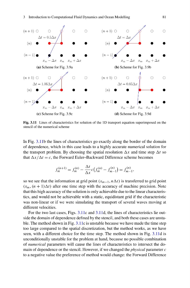
Fig. 3.11 Lines of characteristics for solution of the 1D transport equation superimposed on the
stencil of the numerical scheme
In Fig. 3.11b the lines of characteristics go exactly along the border of the domain
of dependence, which in this case leads to a highly accurate numerical solution for
the transport problem. By choosing the spatial resolution x and time step t so
that = c, the Forward Euler–Backward Difference scheme becomes
f
(n+1)
m
= f
(n)
m −
t
x
c
f
(n)
m − f
(n)
m−1
= f
(n)
m−1 ,
so we see that the information at grid point (x m−1 , nnt) is transferred to grid point
(x m , (n + 1))t) after one time step with the accuracy of machine precision. Note
that this high accuracy of the solution is only achievable due to the linear characteristics, and would not be achievable with a static, equidistant grid if the characteristic
was non-linear or if we were simulating the transport of several waves moving at
different velocities.
For the two last cases, Figs. 3.11c and 3.11d, the lines of characteristics lie outside the domain of dependence defined by the stencil, and both these cases are unstable. The method shown in Fig. 3.11c is unstable because we have made the time step
too large compared to the spatial discretization, but the method works, as we have
seen, with a different choice for the time step. The method shown in Fig. 3.11d is
unconditionally unstable for the problem at hand, because no possible combination
of numerical parameters will cause the lines of characteristics to intersect the domain of dependence or the stencil. However, if we changed the physical parameter c
to a negative value the preference of method would change: the Forward Difference
81
Fig. 3.11 Lines of characteristics for solution of the 1D transport equation superimposed on the
stencil of the numerical scheme
In Fig. 3.11b the lines of characteristics go exactly along the border of the domain
of dependence, which in this case leads to a highly accurate numerical solution for
the transport problem. By choosing the spatial resolution x and time step t so
that = c, the Forward Euler–Backward Difference scheme becomes
f
(n+1)
m
= f
(n)
m −
t
x
c
f
(n)
m − f
(n)
m−1
= f
(n)
m−1 ,
so we see that the information at grid point (x m−1 , nnt) is transferred to grid point
(x m , (n + 1))t) after one time step with the accuracy of machine precision. Note
that this high accuracy of the solution is only achievable due to the linear characteristics, and would not be achievable with a static, equidistant grid if the characteristic
was non-linear or if we were simulating the transport of several waves moving at
different velocities.
For the two last cases, Figs. 3.11c and 3.11d, the lines of characteristics lie outside the domain of dependence defined by the stencil, and both these cases are unstable. The method shown in Fig. 3.11c is unstable because we have made the time step
too large compared to the spatial discretization, but the method works, as we have
seen, with a different choice for the time step. The method shown in Fig. 3.11d is
unconditionally unstable for the problem at hand, because no possible combination
of numerical parameters will cause the lines of characteristics to intersect the domain of dependence or the stencil. However, if we changed the physical parameter c
to a negative value the preference of method would change: the Forward Difference