

82
T. Torsvik
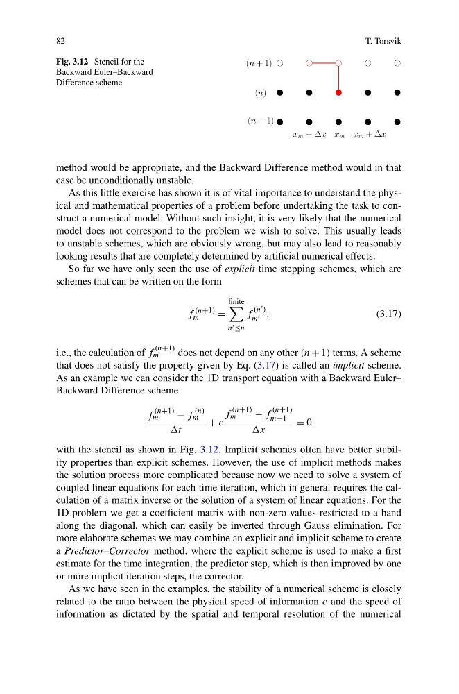
Fig. 3.12 Stencil for the
Backward Euler–Backward
Difference scheme
method would be appropriate, and the Backward Difference method would in that
case be unconditionally unstable.
As this little exercise has shown it is of vital importance to understand the physical and mathematical properties of a problem before undertaking the task to construct a numerical model. Without such insight, it is very likely that the numerical
model does not correspond to the problem we wish to solve. This usually leads
to unstable schemes, which are obviously wrong, but may also lead to reasonably
looking results that are completely determined by artificial numerical effects.
So far we have only seen the use of explicit time stepping schemes, which are
schemes that can be written on the form
f
(n+1)
m
=
finite
n ≤n
f
(n )
m ,
(3.17)
i.e., the calculation of f
(n+1)
m
does not depend on any other (n + 1) terms. A scheme
that does not satisfy the property given by Eq. (3.17) is called an implicit scheme.
As an example we can consider the 1D transport equation with a Backward Euler–
Backward Difference scheme
f
(n+1)
m
− f
(n)
m
t
+ c
f
(n+1)
m
− f
(n+1)
m−1
x
= 0
with the stencil as shown in Fig. 3.12. Implicit schemes often have better stability properties than explicit schemes. However, the use of implicit methods makes
the solution process more complicated because now we need to solve a system of
coupled linear equations for each time iteration, which in general requires the calculation of a matrix inverse or the solution of a system of linear equations. For the
1D problem we get a coefficient matrix with non-zero values restricted to a band
along the diagonal, which can easily be inverted through Gauss elimination. For
more elaborate schemes we may combine an explicit and implicit scheme to create
a Predictor–Corrector method, where the explicit scheme is used to make a first
estimate for the time integration, the predictor step, which is then improved by one
or more implicit iteration steps, the corrector.
As we have seen in the examples, the stability of a numerical scheme is closely
related to the ratio between the physical speed of information c and the speed of
information as dictated by the spatial and temporal resolution of the numerical
T. Torsvik
Fig. 3.12 Stencil for the
Backward Euler–Backward
Difference scheme
method would be appropriate, and the Backward Difference method would in that
case be unconditionally unstable.
As this little exercise has shown it is of vital importance to understand the physical and mathematical properties of a problem before undertaking the task to construct a numerical model. Without such insight, it is very likely that the numerical
model does not correspond to the problem we wish to solve. This usually leads
to unstable schemes, which are obviously wrong, but may also lead to reasonably
looking results that are completely determined by artificial numerical effects.
So far we have only seen the use of explicit time stepping schemes, which are
schemes that can be written on the form
f
(n+1)
m
=
finite
n ≤n
f
(n )
m ,
(3.17)
i.e., the calculation of f
(n+1)
m
does not depend on any other (n + 1) terms. A scheme
that does not satisfy the property given by Eq. (3.17) is called an implicit scheme.
As an example we can consider the 1D transport equation with a Backward Euler–
Backward Difference scheme
f
(n+1)
m
− f
(n)
m
t
+ c
f
(n+1)
m
− f
(n+1)
m−1
x
= 0
with the stencil as shown in Fig. 3.12. Implicit schemes often have better stability properties than explicit schemes. However, the use of implicit methods makes
the solution process more complicated because now we need to solve a system of
coupled linear equations for each time iteration, which in general requires the calculation of a matrix inverse or the solution of a system of linear equations. For the
1D problem we get a coefficient matrix with non-zero values restricted to a band
along the diagonal, which can easily be inverted through Gauss elimination. For
more elaborate schemes we may combine an explicit and implicit scheme to create
a Predictor–Corrector method, where the explicit scheme is used to make a first
estimate for the time integration, the predictor step, which is then improved by one
or more implicit iteration steps, the corrector.
As we have seen in the examples, the stability of a numerical scheme is closely
related to the ratio between the physical speed of information c and the speed of
information as dictated by the spatial and temporal resolution of the numerical