

80
T. Torsvik
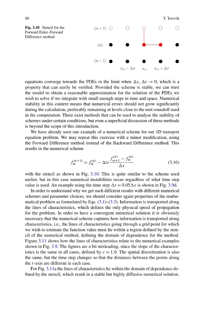
Fig. 3.10 Stencil for the
Forward Euler–Forward
Difference method
equations converge towards the PDEs in the limit when ,t → 0, which is a
property that can easily be verified. Provided the scheme is stable, we can trust
the model to obtain a reasonable approximation for the solution of the PDEs we
wish to solve if we integrate with small enough steps in time and space. Numerical
stability in this context means that numerical errors should not grow significantly
during the calculation, preferably remaining at levels close to the unit roundoff used
in the computation. There exist methods that can be used to analyse the stability of
schemes under certain conditions, but even a superficial discussion of these methods
is beyond the scope of this introduction.
We have already seen one example of a numerical scheme for our 1D transport
equation problem. We may repeat this exercise with a minor modification, using
the Forward Difference method instead of the Backward Difference method. This
results in the numerical scheme
f
(n+1)
m
= f
(n)
m − tc
f
(n)
m+1 − f
(n)
m
x
(3.16)
with the stencil as shown in Fig. 3.10. This is quite similar to the scheme used
earlier, but in this case numerical instabilities occur regardless of what time step
value is used. An example using the time step t = 0.05x is shown in Fig. 3.9d.
In order to understand why we get such different results with different numerical
schemes and parameter choices, we should consider again properties of the mathematical problem as formulated by Eqs. (3.1)–(3.3). Information is transported along
the lines of characteristics, which defines the only physical speed of propagation
for the problem. In order to have a convergent numerical solution it is obviously
necessary that the numerical scheme captures how information is transported along
characteristics, i.e., the lines of characteristics going through a grid point for which
we wish to estimate the function value must lie within a region defined by the stencil of the numerical method, defining the domain of dependence for the method.
Figure 3.11 shows how the lines of characteristics relate to the numerical examples
shown in Fig. 3.9. The figures are a bit misleading, since the slope of the characteristics is the same in all cases, defined by c = 1.0. The spatial discretization is also
the same, but the time step changes so that the distances between the points along
the t-axis are different in each case.
For Fig. 3.11a the lines of characteristics lie within the domain of dependence defined by the stencil, which result in a stable but highly diffusive numerical solution.
T. Torsvik
Fig. 3.10 Stencil for the
Forward Euler–Forward
Difference method
equations converge towards the PDEs in the limit when ,t → 0, which is a
property that can easily be verified. Provided the scheme is stable, we can trust
the model to obtain a reasonable approximation for the solution of the PDEs we
wish to solve if we integrate with small enough steps in time and space. Numerical
stability in this context means that numerical errors should not grow significantly
during the calculation, preferably remaining at levels close to the unit roundoff used
in the computation. There exist methods that can be used to analyse the stability of
schemes under certain conditions, but even a superficial discussion of these methods
is beyond the scope of this introduction.
We have already seen one example of a numerical scheme for our 1D transport
equation problem. We may repeat this exercise with a minor modification, using
the Forward Difference method instead of the Backward Difference method. This
results in the numerical scheme
f
(n+1)
m
= f
(n)
m − tc
f
(n)
m+1 − f
(n)
m
x
(3.16)
with the stencil as shown in Fig. 3.10. This is quite similar to the scheme used
earlier, but in this case numerical instabilities occur regardless of what time step
value is used. An example using the time step t = 0.05x is shown in Fig. 3.9d.
In order to understand why we get such different results with different numerical
schemes and parameter choices, we should consider again properties of the mathematical problem as formulated by Eqs. (3.1)–(3.3). Information is transported along
the lines of characteristics, which defines the only physical speed of propagation
for the problem. In order to have a convergent numerical solution it is obviously
necessary that the numerical scheme captures how information is transported along
characteristics, i.e., the lines of characteristics going through a grid point for which
we wish to estimate the function value must lie within a region defined by the stencil of the numerical method, defining the domain of dependence for the method.
Figure 3.11 shows how the lines of characteristics relate to the numerical examples
shown in Fig. 3.9. The figures are a bit misleading, since the slope of the characteristics is the same in all cases, defined by c = 1.0. The spatial discretization is also
the same, but the time step changes so that the distances between the points along
the t-axis are different in each case.
For Fig. 3.11a the lines of characteristics lie within the domain of dependence defined by the stencil, which result in a stable but highly diffusive numerical solution.