

3 Introduction to Computational Fluid Dynamics and Ocean Modelling
79
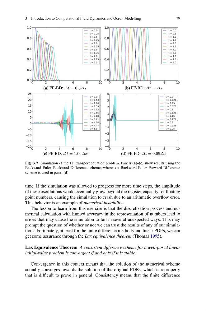
Fig. 3.9 Simulation of the 1D transport equation problem. Panels (a)–(c) show results using the
Backward Euler–Backward Difference scheme, whereas a Backward Euler–Forward Difference
scheme is used in panel (d)
time. If the simulation was allowed to progress for more time steps, the amplitude
of these oscillations would eventually grow beyond the register capacity for floating
point numbers, causing the simulation to crash due to an arithmetic overflow error.
This behavior is an example of numerical instability.
The lesson to learn from this exercise is that the discretization process and numerical calculation with limited accuracy in the representation of numbers lead to
errors that may cause the simulation to fail in several unexpected ways. This may
prompt the question of whether or not we can trust the results of any of our simulations. Fortunately, at least for the finite difference methods and linear PDEs, we can
get some assurance through the Lax equivalence theorem (Thomas 1995).
Lax Equivalence Theorem A consistent difference scheme for a well-posed linear
initial-value problem is convergent if and only if it is stable.
Convergence in this context means that the solution of the numerical scheme
actually converges towards the solution of the original PDEs, which is a property
that is difficult to prove in general. Consistency means that the finite difference
79
Fig. 3.9 Simulation of the 1D transport equation problem. Panels (a)–(c) show results using the
Backward Euler–Backward Difference scheme, whereas a Backward Euler–Forward Difference
scheme is used in panel (d)
time. If the simulation was allowed to progress for more time steps, the amplitude
of these oscillations would eventually grow beyond the register capacity for floating
point numbers, causing the simulation to crash due to an arithmetic overflow error.
This behavior is an example of numerical instability.
The lesson to learn from this exercise is that the discretization process and numerical calculation with limited accuracy in the representation of numbers lead to
errors that may cause the simulation to fail in several unexpected ways. This may
prompt the question of whether or not we can trust the results of any of our simulations. Fortunately, at least for the finite difference methods and linear PDEs, we can
get some assurance through the Lax equivalence theorem (Thomas 1995).
Lax Equivalence Theorem A consistent difference scheme for a well-posed linear
initial-value problem is convergent if and only if it is stable.
Convergence in this context means that the solution of the numerical scheme
actually converges towards the solution of the original PDEs, which is a property
that is difficult to prove in general. Consistency means that the finite difference