

76
T. Torsvik
derivative by combining Eq. (3.6) and Eq. (3.8) in a way that eliminates the 1st order
derivative term
∂ 2 f
(n)
m
∂x 2 ≈
f
(n)
m+1 − 2f
(n)
m + f
(n−1)
m
x 2
,
(3.11)
where the LTE is given by
x 2
24
∂ 4 f
(n)
m
∂x 4 = O
x
2
.
Finite differences for time derivatives can be constructed in the same way as for
the space derivatives, by replacing derivatives in space with derivatives in time, and
replacing x by t. For instance, the Forward Euler method
∂f
(n)
m
∂t
≈
f
(n+1)
m
− f
(n)
m
t
(3.12)
and Backward Euler method
∂f
(n)
m
∂t
≈
f
(n)
m − f
(n−1)
m
t
(3.13)
are direct time derivative analogs to the forward difference and backward difference
methods, respectively. Although the principles for obtaining the finite difference
approximations are the same in space and time, time differentiation usually involves
unknown function values, i.e., we may know the function values for all times up
to and including the terms f
(n)
m , whereas the function values f
(n+1)
m
are unknown.
Higher order methods and approximations for higher order time derivatives may
therefore involve several terms backward in time but will as a rule not involve terms
beyond the first unknown time step.
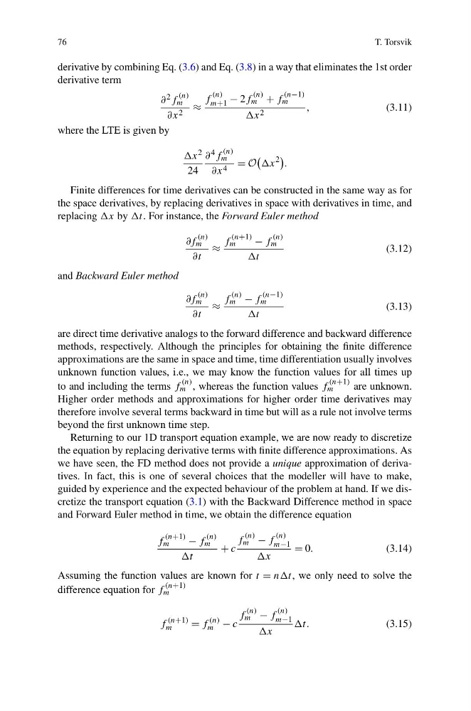
Returning to our 1D transport equation example, we are now ready to discretize
the equation by replacing derivative terms with finite difference approximations. As
we have seen, the FD method does not provide a unique approximation of derivatives. In fact, this is one of several choices that the modeller will have to make,
guided by experience and the expected behaviour of the problem at hand. If we discretize the transport equation (3.1) with the Backward Difference method in space
and Forward Euler method in time, we obtain the difference equation
f
(n+1)
m
− f
(n)
m
t
+ c
f
(n)
m − f
(n)
m−1
x
= 0.
(3.14)
Assuming the function values are known for t = nnt, we only need to solve the
difference equation for f
(n+1)
m
f
(n+1)
m
= f
(n)
m − c
f
(n)
m − f
(n)
m−1
x
t.
(3.15)
T. Torsvik
derivative by combining Eq. (3.6) and Eq. (3.8) in a way that eliminates the 1st order
derivative term
∂ 2 f
(n)
m
∂x 2 ≈
f
(n)
m+1 − 2f
(n)
m + f
(n−1)
m
x 2
,
(3.11)
where the LTE is given by
x 2
24
∂ 4 f
(n)
m
∂x 4 = O
x
2
.
Finite differences for time derivatives can be constructed in the same way as for
the space derivatives, by replacing derivatives in space with derivatives in time, and
replacing x by t. For instance, the Forward Euler method
∂f
(n)
m
∂t
≈
f
(n+1)
m
− f
(n)
m
t
(3.12)
and Backward Euler method
∂f
(n)
m
∂t
≈
f
(n)
m − f
(n−1)
m
t
(3.13)
are direct time derivative analogs to the forward difference and backward difference
methods, respectively. Although the principles for obtaining the finite difference
approximations are the same in space and time, time differentiation usually involves
unknown function values, i.e., we may know the function values for all times up
to and including the terms f
(n)
m , whereas the function values f
(n+1)
m
are unknown.
Higher order methods and approximations for higher order time derivatives may
therefore involve several terms backward in time but will as a rule not involve terms
beyond the first unknown time step.
Returning to our 1D transport equation example, we are now ready to discretize
the equation by replacing derivative terms with finite difference approximations. As
we have seen, the FD method does not provide a unique approximation of derivatives. In fact, this is one of several choices that the modeller will have to make,
guided by experience and the expected behaviour of the problem at hand. If we discretize the transport equation (3.1) with the Backward Difference method in space
and Forward Euler method in time, we obtain the difference equation
f
(n+1)
m
− f
(n)
m
t
+ c
f
(n)
m − f
(n)
m−1
x
= 0.
(3.14)
Assuming the function values are known for t = nnt, we only need to solve the
difference equation for f
(n+1)
m
f
(n+1)
m
= f
(n)
m − c
f
(n)
m − f
(n)
m−1
x
t.
(3.15)