

3 Introduction to Computational Fluid Dynamics and Ocean Modelling
75
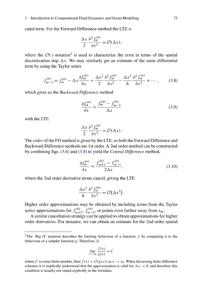
cated term. For the Forward Difference method the LTE is
x
2
∂ 2 f
(n)
m
∂x 2 = O((x),
where the O(·) notation 2 is used to characterize the error in terms of the spatial
discretization step x. We may similarly get an estimate of the same differential
term by using the Taylor series
f
(n)
m−1 = f
(n)
m − x
∂f
(n)
m
∂x
+
x 2
2
∂ 2 f
(n)
m
∂x 2 −
x 3
6
∂ 3 f
(n)
m
∂x 3 + · · · ,
(3.8)
which gives us the Backward Difference method
∂f
(n)
m
∂x
≈
f
(n)
m − f
(n)
m−1
x
(3.9)
with the LTE
x
2
∂ 2 f
(n)
m
∂x 2 = O((x).
The order of the FD method is given by the LTE, so both the Forward Difference and
Backward Difference methods are 1st order. A 2nd order method can be constructed
by combining Eqs. (3.6) and (3.8) to yield the Central Difference method,
∂f
(n)
m
∂x
≈
f
(n)
m+1 − f
(n)
m−1
2x
,
(3.10)
where the 2nd order derivative terms cancel, giving the LTE
x 2
6
∂ 3 f
(n)
m
∂x 3 = O
x
2
.
Higher order approximations may be obtained by including terms from the Taylor
series approximations for f
(n)
m+2 , f
(n)
m−2 , or points even further away from x m .
A similar cancellation strategy can be applied to obtain approximations for higher
order derivatives. For instance, we can obtain an estimate for the 2nd order spatial
2 The ‘Big O’ notation describes the limiting behaviour of a function f by comparing it to the
behaviour of a simpler function g. Therefore, if
lim
x→x 0
f (x)
g(x)
= C
where C is some finite number, then f (x) = O(g(x)) as x → x 0 . When discussing finite difference
schemes it is implicitly understood that the approximation is valid for x → 0, and therefore this
condition is usually not stated explicitly in the formulas.
75
cated term. For the Forward Difference method the LTE is
x
2
∂ 2 f
(n)
m
∂x 2 = O((x),
where the O(·) notation 2 is used to characterize the error in terms of the spatial
discretization step x. We may similarly get an estimate of the same differential
term by using the Taylor series
f
(n)
m−1 = f
(n)
m − x
∂f
(n)
m
∂x
+
x 2
2
∂ 2 f
(n)
m
∂x 2 −
x 3
6
∂ 3 f
(n)
m
∂x 3 + · · · ,
(3.8)
which gives us the Backward Difference method
∂f
(n)
m
∂x
≈
f
(n)
m − f
(n)
m−1
x
(3.9)
with the LTE
x
2
∂ 2 f
(n)
m
∂x 2 = O((x).
The order of the FD method is given by the LTE, so both the Forward Difference and
Backward Difference methods are 1st order. A 2nd order method can be constructed
by combining Eqs. (3.6) and (3.8) to yield the Central Difference method,
∂f
(n)
m
∂x
≈
f
(n)
m+1 − f
(n)
m−1
2x
,
(3.10)
where the 2nd order derivative terms cancel, giving the LTE
x 2
6
∂ 3 f
(n)
m
∂x 3 = O
x
2
.
Higher order approximations may be obtained by including terms from the Taylor
series approximations for f
(n)
m+2 , f
(n)
m−2 , or points even further away from x m .
A similar cancellation strategy can be applied to obtain approximations for higher
order derivatives. For instance, we can obtain an estimate for the 2nd order spatial
2 The ‘Big O’ notation describes the limiting behaviour of a function f by comparing it to the
behaviour of a simpler function g. Therefore, if
lim
x→x 0
f (x)
g(x)
= C
where C is some finite number, then f (x) = O(g(x)) as x → x 0 . When discussing finite difference
schemes it is implicitly understood that the approximation is valid for x → 0, and therefore this
condition is usually not stated explicitly in the formulas.