

3 Introduction to Computational Fluid Dynamics and Ocean Modelling
77
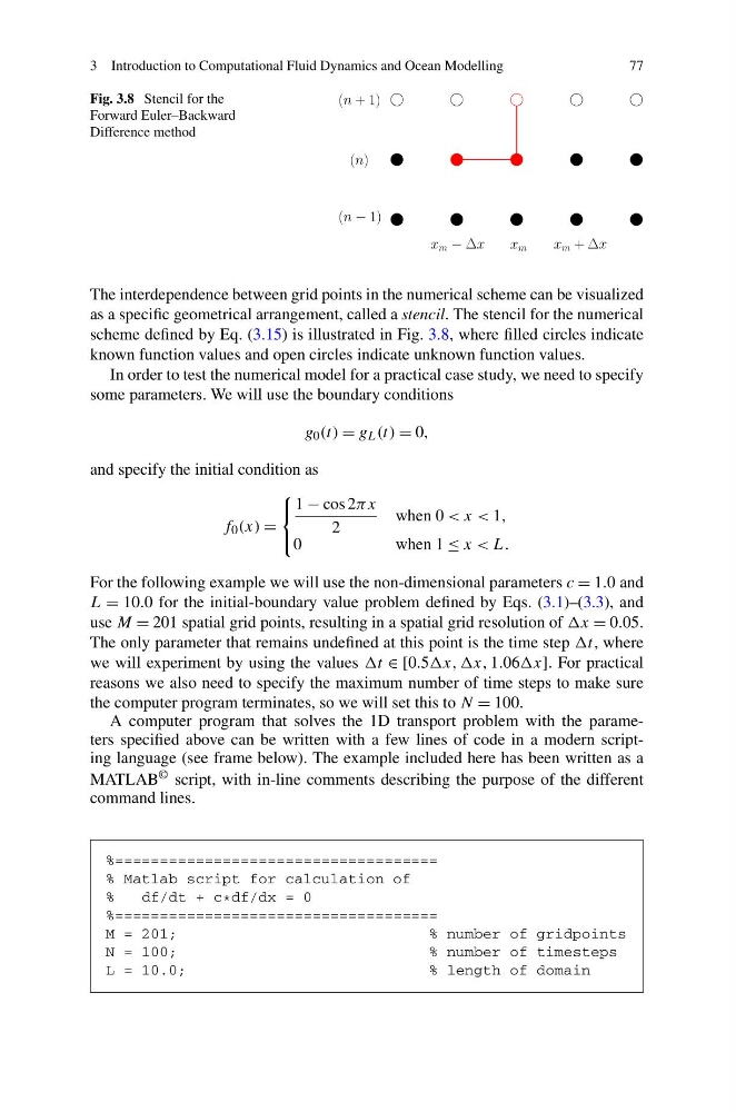
Fig. 3.8 Stencil for the
Forward Euler–Backward
Difference method
The interdependence between grid points in the numerical scheme can be visualized
as a specific geometrical arrangement, called a stencil. The stencil for the numerical
scheme defined by Eq. (3.15) is illustrated in Fig. 3.8, where filled circles indicate
known function values and open circles indicate unknown function values.
In order to test the numerical model for a practical case study, we need to specify
some parameters. We will use the boundary conditions
g 0 (t) = g L (t) = 0,
and specify the initial condition as
f 0 (x) =
⎧
⎨
⎩
1 − cos 2πx
2
when 0 < x < 1,
0
when 1 ≤ x < L.
For the following example we will use the non-dimensional parameters c = 1.0 and
L = 10.0 for the initial-boundary value problem defined by Eqs. (3.1)–(3.3), and
use M = 201 spatial grid points, resulting in a spatial grid resolution of x = 0.05.
The only parameter that remains undefined at this point is the time step t, where
we will experiment by using the values t ∈ [0.5x, ,x, 1.06x]. For practical
reasons we also need to specify the maximum number of time steps to make sure
the computer program terminates, so we will set this to N = 100.
A computer program that solves the 1D transport problem with the parameters specified above can be written with a few lines of code in a modern scripting language (see frame below). The example included here has been written as a
MATLAB © script, with in-line comments describing the purpose of the different
command lines.
%====================================
% Matlab script for calculation of
%
df/dt + c * df/dx = 0
%====================================
M = 201;
% number of gridpoints
N = 100;
% number of timesteps
L = 10.0;
% length of domain
77
Fig. 3.8 Stencil for the
Forward Euler–Backward
Difference method
The interdependence between grid points in the numerical scheme can be visualized
as a specific geometrical arrangement, called a stencil. The stencil for the numerical
scheme defined by Eq. (3.15) is illustrated in Fig. 3.8, where filled circles indicate
known function values and open circles indicate unknown function values.
In order to test the numerical model for a practical case study, we need to specify
some parameters. We will use the boundary conditions
g 0 (t) = g L (t) = 0,
and specify the initial condition as
f 0 (x) =
⎧
⎨
⎩
1 − cos 2πx
2
when 0 < x < 1,
0
when 1 ≤ x < L.
For the following example we will use the non-dimensional parameters c = 1.0 and
L = 10.0 for the initial-boundary value problem defined by Eqs. (3.1)–(3.3), and
use M = 201 spatial grid points, resulting in a spatial grid resolution of x = 0.05.
The only parameter that remains undefined at this point is the time step t, where
we will experiment by using the values t ∈ [0.5x, ,x, 1.06x]. For practical
reasons we also need to specify the maximum number of time steps to make sure
the computer program terminates, so we will set this to N = 100.
A computer program that solves the 1D transport problem with the parameters specified above can be written with a few lines of code in a modern scripting language (see frame below). The example included here has been written as a
MATLAB © script, with in-line comments describing the purpose of the different
command lines.
%====================================
% Matlab script for calculation of
%
df/dt + c * df/dx = 0
%====================================
M = 201;
% number of gridpoints
N = 100;
% number of timesteps
L = 10.0;
% length of domain