

72
T. Torsvik
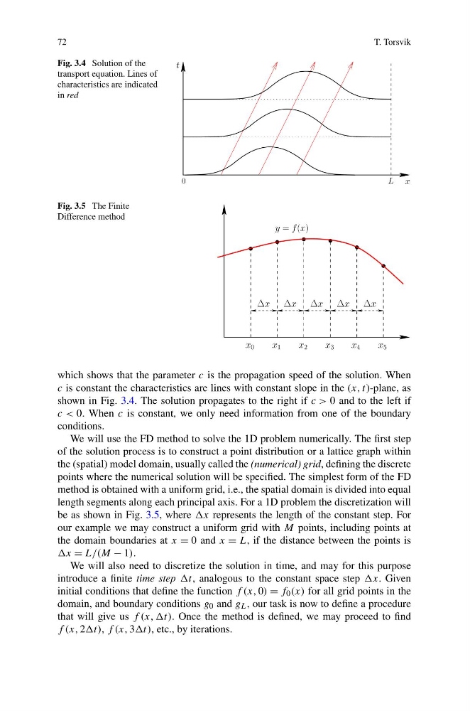
Fig. 3.4 Solution of the
transport equation. Lines of
characteristics are indicated
in red
Fig. 3.5 The Finite
Difference method
which shows that the parameter c is the propagation speed of the solution. When
c is constant the characteristics are lines with constant slope in the (x, t)-plane, as
shown in Fig. 3.4. The solution propagates to the right if c > 0 and to the left if
c < 0. When c is constant, we only need information from one of the boundary
conditions.
We will use the FD method to solve the 1D problem numerically. The first step
of the solution process is to construct a point distribution or a lattice graph within
the (spatial) model domain, usually called the (numerical) grid, defining the discrete
points where the numerical solution will be specified. The simplest form of the FD
method is obtained with a uniform grid, i.e., the spatial domain is divided into equal
length segments along each principal axis. For a 1D problem the discretization will
be as shown in Fig. 3.5, where x represents the length of the constant step. For
our example we may construct a uniform grid with M points, including points at
the domain boundaries at x = 0 and x = L, if the distance between the points is
x = L/(M − 1).
We will also need to discretize the solution in time, and may for this purpose
introduce a finite time step t, analogous to the constant space step x. Given
initial conditions that define the function f (x, 0) = f 0 (x) for all grid points in the
domain, and boundary conditions g 0 and g L , our task is now to define a procedure
that will give us f (x, ,t). Once the method is defined, we may proceed to find
f (x, 2 f (x, 3 etc., by iterations.
T. Torsvik
Fig. 3.4 Solution of the
transport equation. Lines of
characteristics are indicated
in red
Fig. 3.5 The Finite
Difference method
which shows that the parameter c is the propagation speed of the solution. When
c is constant the characteristics are lines with constant slope in the (x, t)-plane, as
shown in Fig. 3.4. The solution propagates to the right if c > 0 and to the left if
c < 0. When c is constant, we only need information from one of the boundary
conditions.
We will use the FD method to solve the 1D problem numerically. The first step
of the solution process is to construct a point distribution or a lattice graph within
the (spatial) model domain, usually called the (numerical) grid, defining the discrete
points where the numerical solution will be specified. The simplest form of the FD
method is obtained with a uniform grid, i.e., the spatial domain is divided into equal
length segments along each principal axis. For a 1D problem the discretization will
be as shown in Fig. 3.5, where x represents the length of the constant step. For
our example we may construct a uniform grid with M points, including points at
the domain boundaries at x = 0 and x = L, if the distance between the points is
x = L/(M − 1).
We will also need to discretize the solution in time, and may for this purpose
introduce a finite time step t, analogous to the constant space step x. Given
initial conditions that define the function f (x, 0) = f 0 (x) for all grid points in the
domain, and boundary conditions g 0 and g L , our task is now to define a procedure
that will give us f (x, ,t). Once the method is defined, we may proceed to find
f (x, 2 f (x, 3 etc., by iterations.