

3 Introduction to Computational Fluid Dynamics and Ocean Modelling
71
Anderson (1995) with focus on the FD method, and Ferziger and Peri´ c (2002)
which includes discussions on the FD and FV methods, can both be recommended. A useful resource for CFD-related topics is the web site CFD Online
(http://www.cfd-online.com), which includes overviews of CFD software and literature, discussion forums and an overview of conferences and workshops. For
introduction level books on numerical methods, Thomas (1995), LeVeque (2002)
and Johnson (2009) can be recommended for the FD method, FV method and FE
method, respectively.
3.2.2 The Finite Difference Method
This short introduction is not intended as an exposition of fundamental theory or
advanced CFD methods. We will instead focus on simple methods that demonstrate
some general concepts of numerical modelling. For this purpose we will now do a
step by step demonstration of how to construct a simple numerical model, and leave
the discussion of more general topics for later. This part is intended for readers with
no previous experience with numerical models.
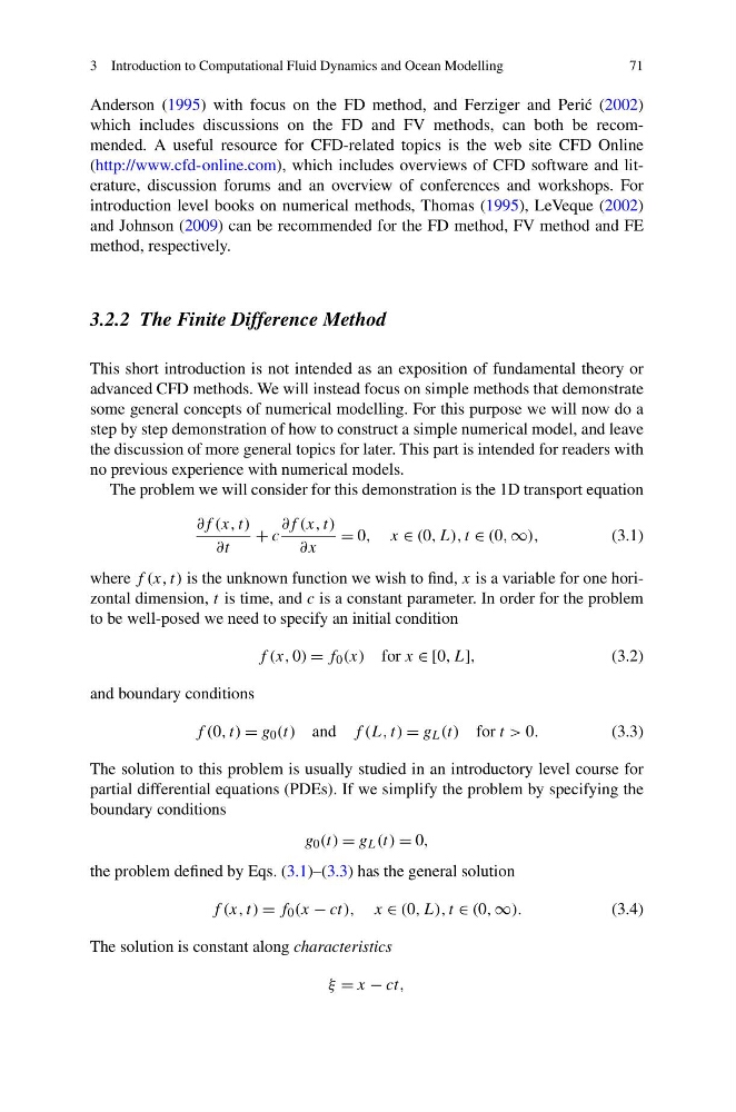
The problem we will consider for this demonstration is the 1D transport equation
∂f (x, t)
∂t
+ c
∂f (x, t)
∂x
= 0, x ∈ (0, L), t ∈ (0, ∞),
(3.1)
where f (x, t) is the unknown function we wish to find, x is a variable for one horizontal dimension, t is time, and c is a constant parameter. In order for the problem
to be well-posed we need to specify an initial condition
f (x, 0) = f 0 (x) for x ∈ [0, L],
(3.2)
and boundary conditions
f (0, t) = g 0 (t) and f (L, t) = g L (t) for t > 0.
(3.3)
The solution to this problem is usually studied in an introductory level course for
partial differential equations (PDEs). If we simplify the problem by specifying the
boundary conditions
g 0 (t) = g L (t) = 0,
the problem defined by Eqs. (3.1)–(3.3) has the general solution
f (x, t) = f 0 (x − ct), x ∈ (0, L), t ∈ (0, ∞).
(3.4)
The solution is constant along characteristics
ξ = x − ct,
71
Anderson (1995) with focus on the FD method, and Ferziger and Peri´ c (2002)
which includes discussions on the FD and FV methods, can both be recommended. A useful resource for CFD-related topics is the web site CFD Online
(http://www.cfd-online.com), which includes overviews of CFD software and literature, discussion forums and an overview of conferences and workshops. For
introduction level books on numerical methods, Thomas (1995), LeVeque (2002)
and Johnson (2009) can be recommended for the FD method, FV method and FE
method, respectively.
3.2.2 The Finite Difference Method
This short introduction is not intended as an exposition of fundamental theory or
advanced CFD methods. We will instead focus on simple methods that demonstrate
some general concepts of numerical modelling. For this purpose we will now do a
step by step demonstration of how to construct a simple numerical model, and leave
the discussion of more general topics for later. This part is intended for readers with
no previous experience with numerical models.
The problem we will consider for this demonstration is the 1D transport equation
∂f (x, t)
∂t
+ c
∂f (x, t)
∂x
= 0, x ∈ (0, L), t ∈ (0, ∞),
(3.1)
where f (x, t) is the unknown function we wish to find, x is a variable for one horizontal dimension, t is time, and c is a constant parameter. In order for the problem
to be well-posed we need to specify an initial condition
f (x, 0) = f 0 (x) for x ∈ [0, L],
(3.2)
and boundary conditions
f (0, t) = g 0 (t) and f (L, t) = g L (t) for t > 0.
(3.3)
The solution to this problem is usually studied in an introductory level course for
partial differential equations (PDEs). If we simplify the problem by specifying the
boundary conditions
g 0 (t) = g L (t) = 0,
the problem defined by Eqs. (3.1)–(3.3) has the general solution
f (x, t) = f 0 (x − ct), x ∈ (0, L), t ∈ (0, ∞).
(3.4)
The solution is constant along characteristics
ξ = x − ct,