

3 Introduction to Computational Fluid Dynamics and Ocean Modelling
73
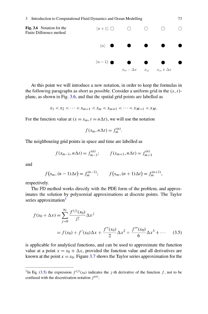
Fig. 3.6 Notation for the
Finite Difference method
At this point we will introduce a new notation, in order to keep the formulas in
the following paragraphs as short as possible. Consider a uniform grid in the (x, t)plane, as shown in Fig. 3.6, and that the spatial grid points are labelled as
x 1 < x 2 < · · · < x m−1 < x m < x m+1 < · · · < x M−1 < x M .
For the function value at (x = x m , t = nnt), we will use the notation
f (x m , nnt) = f
(n)
m .
The neighbouring grid points in space and time are labelled as
f (x m−1 , nnt) = f
(n)
m−1 ;
f (x m+1 , nnt) = f
(n)
m+1
and
f
x m , (n − 1))t
= f
(n−1)
m
;
f
x m , (n + 1))t
= f
(n+1)
m
,
respectively.
The FD method works directly with the PDE form of the problem, and approximates the solution by polynomial approximations at discrete points. The Taylor
series approximation 1
f (x 0 + =
∞
j =0
f (j ) (x 0 )
j !
x
j
= f (x 0 ) + f
(x 0 ))x +
f (x 0 )
2
x
2
+
f (x 0 )
6
x
3
+ · · ·
(3.5)
is applicable for analytical functions, and can be used to approximate the function
value at a point x = x 0 + x, provided the function value and all derivatives are
known at the point x = x 0 . Figure 3.7 shows the Taylor series approximation for the
1 In Eq. (3.5) the expression f (j ) (x 0 ) indicates the j -th derivative of the function f , not to be
confused with the discretization notation f (n) .
73
Fig. 3.6 Notation for the
Finite Difference method
At this point we will introduce a new notation, in order to keep the formulas in
the following paragraphs as short as possible. Consider a uniform grid in the (x, t)plane, as shown in Fig. 3.6, and that the spatial grid points are labelled as
x 1 < x 2 < · · · < x m−1 < x m < x m+1 < · · · < x M−1 < x M .
For the function value at (x = x m , t = nnt), we will use the notation
f (x m , nnt) = f
(n)
m .
The neighbouring grid points in space and time are labelled as
f (x m−1 , nnt) = f
(n)
m−1 ;
f (x m+1 , nnt) = f
(n)
m+1
and
f
x m , (n − 1))t
= f
(n−1)
m
;
f
x m , (n + 1))t
= f
(n+1)
m
,
respectively.
The FD method works directly with the PDE form of the problem, and approximates the solution by polynomial approximations at discrete points. The Taylor
series approximation 1
f (x 0 + =
∞
j =0
f (j ) (x 0 )
j !
x
j
= f (x 0 ) + f
(x 0 ))x +
f (x 0 )
2
x
2
+
f (x 0 )
6
x
3
+ · · ·
(3.5)
is applicable for analytical functions, and can be used to approximate the function
value at a point x = x 0 + x, provided the function value and all derivatives are
known at the point x = x 0 . Figure 3.7 shows the Taylor series approximation for the
1 In Eq. (3.5) the expression f (j ) (x 0 ) indicates the j -th derivative of the function f , not to be
confused with the discretization notation f (n) .