

11 Applications of an Oil Drift and Fate Model for Fairway Design
403
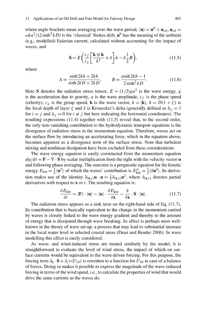
where angle brackets mean averaging over the wave period, u = u 0 + u sd , u sd =
ωka 2 /(2 sinh
2 kD) is the ‘classical’ Stokes drift, u 0 has the meaning of the ambient
(e.g., modelled) Eulerian current, calculated without accounting for the impact of
waves, and
S = E
c f
c g
k ⊗ k
k 2 + δ
A − δ
1
2
B
,
(11.5)
where
A =
sinh 2kh + 2kh
sinh 2kD + 2kD
,
B=
cosh 2kh − 1
2 sinh
2 kD
.
(11.6)
Here S denotes the radiation stress tensor, E = (1/2)ga 2 is the wave energy, g
is the acceleration due to gravity, a is the wave amplitude, c f is the phase speed
(celerity), c g is the group speed, k is the wave vector, k = |k|, h = D(1 + ζ ) is
the local depth of layer ζ and δ is Kronecker’s delta (generally defined as δ ij = 1
for i = j and δ ij = 0 for i = j but here indicating the horizontal coordinates). The
resulting expressions (11.4) together with (11.5) reveal that, to the second order,
the only non-vanishing contribution to the hydrodynamic transport equations is the
divergence of radiation stress in the momentum equation. Therefore, waves act on
the surface flow by introducing an accelerating force, which in the equation above,
becomes apparent as a divergence term of the surface stress. Note that turbulent
mixing and nonlinear dissipation have been excluded from these considerations.
The wave energy equation is easily constructed from the momentum equation
du/dt = F − ∇ · S by scalar multiplication from the right with the velocity vector u
and following phase averaging. The outcome is a prognostic equation for the kinetic
energy E kin =
1
2 u 2 of which the waves’ contribution is E w
kin =
1
2 δu 2 . Its derivation makes use of the identity ∂ (x,t) u · u =
1
2 ∂ (x,t) u 2 , where ∂ (x,t) denotes partial
derivatives with respect to x or t. The resulting equation is:
∂E kin
∂t
= =F · ·u − −u ·
∂E kin
∂x
−
∂
∂x
· S · ·u.
(11.7)
The radiation stress appears as a sink term on the right-hand side of Eq. (11.7).
Its contribution that is basically equivalent to the change in the momentum carried
by waves is closely linked to the wave energy gradient and thereby to the amount
of energy that is dissipated through wave breaking. Its effect is perhaps most wellknown in the theory of wave set-up, a process that may lead to substantial increase
in the local water level in selected coastal areas (Dean and Bender 2006). In wave
modelling this effect is rarely considered.
As wave- and wind-induced stress are treated similarly by the model, it is
straightforward to evaluate the level of wind stress, the impact of which on surface currents would be equivalent to the wave-driven forcing. For this purpose, the
forcing term ∂ x · S + ∂ z τ (U 10 ) is rewritten to a function for U 10 in case of a balance
of forces. Doing so makes it possible to express the magnitude of the wave-induced
forcing in terms of the wind speed, i.e., to calculate the properties of wind that would
drive the same currents as the waves do.
403
where angle brackets mean averaging over the wave period, u = u 0 + u sd , u sd =
ωka 2 /(2 sinh
2 kD) is the ‘classical’ Stokes drift, u 0 has the meaning of the ambient
(e.g., modelled) Eulerian current, calculated without accounting for the impact of
waves, and
S = E
c f
c g
k ⊗ k
k 2 + δ
A − δ
1
2
B
,
(11.5)
where
A =
sinh 2kh + 2kh
sinh 2kD + 2kD
,
B=
cosh 2kh − 1
2 sinh
2 kD
.
(11.6)
Here S denotes the radiation stress tensor, E = (1/2)ga 2 is the wave energy, g
is the acceleration due to gravity, a is the wave amplitude, c f is the phase speed
(celerity), c g is the group speed, k is the wave vector, k = |k|, h = D(1 + ζ ) is
the local depth of layer ζ and δ is Kronecker’s delta (generally defined as δ ij = 1
for i = j and δ ij = 0 for i = j but here indicating the horizontal coordinates). The
resulting expressions (11.4) together with (11.5) reveal that, to the second order,
the only non-vanishing contribution to the hydrodynamic transport equations is the
divergence of radiation stress in the momentum equation. Therefore, waves act on
the surface flow by introducing an accelerating force, which in the equation above,
becomes apparent as a divergence term of the surface stress. Note that turbulent
mixing and nonlinear dissipation have been excluded from these considerations.
The wave energy equation is easily constructed from the momentum equation
du/dt = F − ∇ · S by scalar multiplication from the right with the velocity vector u
and following phase averaging. The outcome is a prognostic equation for the kinetic
energy E kin =
1
2 u 2 of which the waves’ contribution is E w
kin =
1
2 δu 2 . Its derivation makes use of the identity ∂ (x,t) u · u =
1
2 ∂ (x,t) u 2 , where ∂ (x,t) denotes partial
derivatives with respect to x or t. The resulting equation is:
∂E kin
∂t
= =F · ·u − −u ·
∂E kin
∂x
−
∂
∂x
· S · ·u.
(11.7)
The radiation stress appears as a sink term on the right-hand side of Eq. (11.7).
Its contribution that is basically equivalent to the change in the momentum carried
by waves is closely linked to the wave energy gradient and thereby to the amount
of energy that is dissipated through wave breaking. Its effect is perhaps most wellknown in the theory of wave set-up, a process that may lead to substantial increase
in the local water level in selected coastal areas (Dean and Bender 2006). In wave
modelling this effect is rarely considered.
As wave- and wind-induced stress are treated similarly by the model, it is
straightforward to evaluate the level of wind stress, the impact of which on surface currents would be equivalent to the wave-driven forcing. For this purpose, the
forcing term ∂ x · S + ∂ z τ (U 10 ) is rewritten to a function for U 10 in case of a balance
of forces. Doing so makes it possible to express the magnitude of the wave-induced
forcing in terms of the wind speed, i.e., to calculate the properties of wind that would
drive the same currents as the waves do.