

8 Trajectories and Spreading of Observed and Simulated Drifters in the Baltic Sea
267
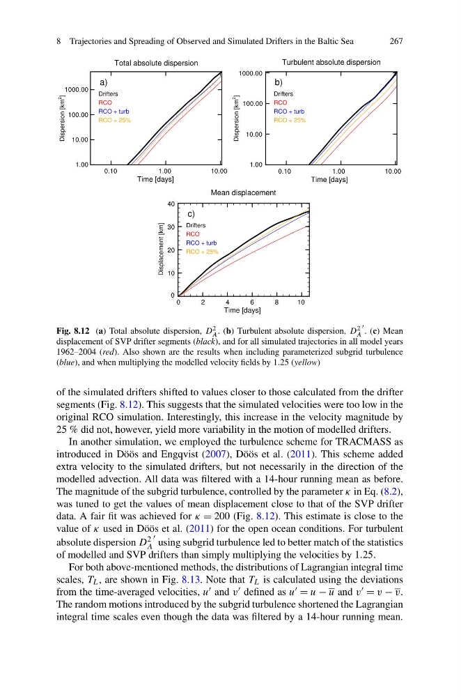
Fig. 8.12 (a) Total absolute dispersion, D 2
A . (b) Turbulent absolute dispersion, D 2
A
. (c) Mean
displacement of SVP drifter segments (black), and for all simulated trajectories in all model years
1962–2004 (red). Also shown are the results when including parameterized subgrid turbulence
(blue), and when multiplying the modelled velocity fields by 1.25 (yellow)
of the simulated drifters shifted to values closer to those calculated from the drifter
segments (Fig. 8.12). This suggests that the simulated velocities were too low in the
original RCO simulation. Interestingly, this increase in the velocity magnitude by
25 % did not, however, yield more variability in the motion of modelled drifters.
In another simulation, we employed the turbulence scheme for TRACMASS as
introduced in Döös and Engqvist (2007), Döös et al. (2011). This scheme added
extra velocity to the simulated drifters, but not necessarily in the direction of the
modelled advection. All data was filtered with a 14-hour running mean as before.
The magnitude of the subgrid turbulence, controlled by the parameter κ in Eq. (8.2),
was tuned to get the values of mean displacement close to that of the SVP drifter
data. A fair fit was achieved for κ = 200 (Fig. 8.12). This estimate is close to the
value of κ used in Döös et al. (2011) for the open ocean conditions. For turbulent
absolute dispersion D 2
A
using subgrid turbulence led to better match of the statistics
of modelled and SVP drifters than simply multiplying the velocities by 1.25.
For both above-mentioned methods, the distributions of Lagrangian integral time
scales, T L , are shown in Fig. 8.13. Note that T L is calculated using the deviations
from the time-averaged velocities, u and v defined as u = u − u and v = v − v.
The random motions introduced by the subgrid turbulence shortened the Lagrangian
integral time scales even though the data was filtered by a 14-hour running mean.
267
Fig. 8.12 (a) Total absolute dispersion, D 2
A . (b) Turbulent absolute dispersion, D 2
A
. (c) Mean
displacement of SVP drifter segments (black), and for all simulated trajectories in all model years
1962–2004 (red). Also shown are the results when including parameterized subgrid turbulence
(blue), and when multiplying the modelled velocity fields by 1.25 (yellow)
of the simulated drifters shifted to values closer to those calculated from the drifter
segments (Fig. 8.12). This suggests that the simulated velocities were too low in the
original RCO simulation. Interestingly, this increase in the velocity magnitude by
25 % did not, however, yield more variability in the motion of modelled drifters.
In another simulation, we employed the turbulence scheme for TRACMASS as
introduced in Döös and Engqvist (2007), Döös et al. (2011). This scheme added
extra velocity to the simulated drifters, but not necessarily in the direction of the
modelled advection. All data was filtered with a 14-hour running mean as before.
The magnitude of the subgrid turbulence, controlled by the parameter κ in Eq. (8.2),
was tuned to get the values of mean displacement close to that of the SVP drifter
data. A fair fit was achieved for κ = 200 (Fig. 8.12). This estimate is close to the
value of κ used in Döös et al. (2011) for the open ocean conditions. For turbulent
absolute dispersion D 2
A
using subgrid turbulence led to better match of the statistics
of modelled and SVP drifters than simply multiplying the velocities by 1.25.
For both above-mentioned methods, the distributions of Lagrangian integral time
scales, T L , are shown in Fig. 8.13. Note that T L is calculated using the deviations
from the time-averaged velocities, u and v defined as u = u − u and v = v − v.
The random motions introduced by the subgrid turbulence shortened the Lagrangian
integral time scales even though the data was filtered by a 14-hour running mean.