

8 Trajectories and Spreading of Observed and Simulated Drifters in the Baltic Sea
265
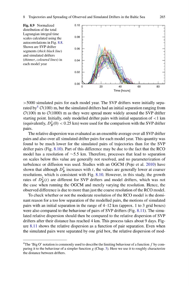
Fig. 8.9 Normalized
distribution of the total
Lagrangian integral time
scales calculated using the
autocorrelations in Fig. 8.8.
Shown are SVP drifter
segments (thick black line)
and simulated drifters
(thinner, coloured lines) in
each model year
>5000 simulated pairs for each model year. The SVP drifters were initially separated by 4 O(100) m, but the simulated drifters had an initial separation ranging from
O(100) m to O(1000) m as they were spread more widely around the SVP drifter
starting point. Initially, only modelled drifter pairs with initial separation of <1 km
(equivalently, D 2
R (0) < 0.25 km) were used for the comparison with the SVP drifter
pairs.
The relative dispersion was evaluated as an ensemble average over all SVP drifter
pairs and also over all simulated drifter pairs for each model year. This quantity was
found to be much lower for the simulated pairs of trajectories than for the SVP
drifter pairs (Fig. 8.10). Part of this difference may be due to the fact that the RCO
model has a resolution of ∼5.5 km. Therefore, processes that lead to separation
on scales below this value are generally not resolved, and no parameterization of
turbulence or diffusion was used. Studies with an OGCM (Poje et al. 2010) have
shown that although D 2
R increases with t, the values are generally lower at coarser
resolutions, which is consistent with Fig. 8.10. However, in this study, the growth
rates of D 2
R (t) are different for SVP drifters and model drifters, which was not
the case when running the OGCM and merely varying the resolution. Hence, the
observed difference is due to more than just the coarse resolution of the RCO model.
To check whether or not the moderate resolution of the RCO model is the dominant reason for a too low separation of the modelled pairs, the motions of simulated
pairs with an initial separation in the range of 4–12 km (approx. 1 to 3 grid boxes)
were also compared to the behaviour of pairs of SVP drifters (Fig. 8.11). The simulated relative dispersion should then be compared to the relative dispersion of SVP
drifters after their distance has reached 4 km. This process takes about 9 days. Figure 8.11 shows the relative dispersion as a function of pair separation. Even when
the simulated pairs were separated by one grid box, the relative dispersion of mod4 The ‘Big O’ notation is commonly used to describe the limiting behaviour of a function f by comparing it to the behaviour of a simpler function g (Chap. 3). Here we use it to roughly characterize
the distance between drifters.
265
Fig. 8.9 Normalized
distribution of the total
Lagrangian integral time
scales calculated using the
autocorrelations in Fig. 8.8.
Shown are SVP drifter
segments (thick black line)
and simulated drifters
(thinner, coloured lines) in
each model year
>5000 simulated pairs for each model year. The SVP drifters were initially separated by 4 O(100) m, but the simulated drifters had an initial separation ranging from
O(100) m to O(1000) m as they were spread more widely around the SVP drifter
starting point. Initially, only modelled drifter pairs with initial separation of <1 km
(equivalently, D 2
R (0) < 0.25 km) were used for the comparison with the SVP drifter
pairs.
The relative dispersion was evaluated as an ensemble average over all SVP drifter
pairs and also over all simulated drifter pairs for each model year. This quantity was
found to be much lower for the simulated pairs of trajectories than for the SVP
drifter pairs (Fig. 8.10). Part of this difference may be due to the fact that the RCO
model has a resolution of ∼5.5 km. Therefore, processes that lead to separation
on scales below this value are generally not resolved, and no parameterization of
turbulence or diffusion was used. Studies with an OGCM (Poje et al. 2010) have
shown that although D 2
R increases with t, the values are generally lower at coarser
resolutions, which is consistent with Fig. 8.10. However, in this study, the growth
rates of D 2
R (t) are different for SVP drifters and model drifters, which was not
the case when running the OGCM and merely varying the resolution. Hence, the
observed difference is due to more than just the coarse resolution of the RCO model.
To check whether or not the moderate resolution of the RCO model is the dominant reason for a too low separation of the modelled pairs, the motions of simulated
pairs with an initial separation in the range of 4–12 km (approx. 1 to 3 grid boxes)
were also compared to the behaviour of pairs of SVP drifters (Fig. 8.11). The simulated relative dispersion should then be compared to the relative dispersion of SVP
drifters after their distance has reached 4 km. This process takes about 9 days. Figure 8.11 shows the relative dispersion as a function of pair separation. Even when
the simulated pairs were separated by one grid box, the relative dispersion of mod4 The ‘Big O’ notation is commonly used to describe the limiting behaviour of a function f by comparing it to the behaviour of a simpler function g (Chap. 3). Here we use it to roughly characterize
the distance between drifters.