

264
J. Kjellsson et al.
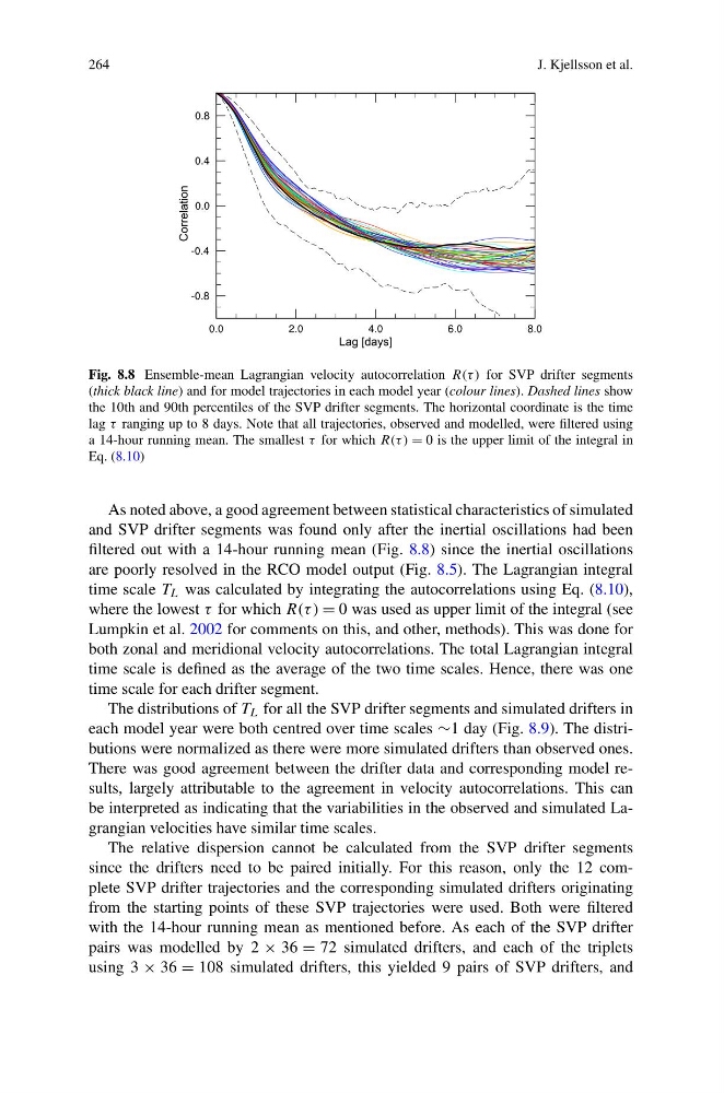
Fig. 8.8 Ensemble-mean Lagrangian velocity autocorrelation R(τ ) for SVP drifter segments
(thick black line) and for model trajectories in each model year (colour lines). Dashed lines show
the 10th and 90th percentiles of the SVP drifter segments. The horizontal coordinate is the time
lag τ ranging up to 8 days. Note that all trajectories, observed and modelled, were filtered using
a 14-hour running mean. The smallest τ for which R(τ ) = 0 is the upper limit of the integral in
Eq. (8.10)
As noted above, a good agreement between statistical characteristics of simulated
and SVP drifter segments was found only after the inertial oscillations had been
filtered out with a 14-hour running mean (Fig. 8.8) since the inertial oscillations
are poorly resolved in the RCO model output (Fig. 8.5). The Lagrangian integral
time scale T L was calculated by integrating the autocorrelations using Eq. (8.10),
where the lowest τ for which R(τ ) = 0 was used as upper limit of the integral (see
Lumpkin et al. 2002 for comments on this, and other, methods). This was done for
both zonal and meridional velocity autocorrelations. The total Lagrangian integral
time scale is defined as the average of the two time scales. Hence, there was one
time scale for each drifter segment.
The distributions of T L for all the SVP drifter segments and simulated drifters in
each model year were both centred over time scales ∼1 day (Fig. 8.9). The distributions were normalized as there were more simulated drifters than observed ones.
There was good agreement between the drifter data and corresponding model results, largely attributable to the agreement in velocity autocorrelations. This can
be interpreted as indicating that the variabilities in the observed and simulated Lagrangian velocities have similar time scales.
The relative dispersion cannot be calculated from the SVP drifter segments
since the drifters need to be paired initially. For this reason, only the 12 complete SVP drifter trajectories and the corresponding simulated drifters originating
from the starting points of these SVP trajectories were used. Both were filtered
with the 14-hour running mean as mentioned before. As each of the SVP drifter
pairs was modelled by 2 × 36 = 72 simulated drifters, and each of the triplets
using 3 × 36 = 108 simulated drifters, this yielded 9 pairs of SVP drifters, and
J. Kjellsson et al.
Fig. 8.8 Ensemble-mean Lagrangian velocity autocorrelation R(τ ) for SVP drifter segments
(thick black line) and for model trajectories in each model year (colour lines). Dashed lines show
the 10th and 90th percentiles of the SVP drifter segments. The horizontal coordinate is the time
lag τ ranging up to 8 days. Note that all trajectories, observed and modelled, were filtered using
a 14-hour running mean. The smallest τ for which R(τ ) = 0 is the upper limit of the integral in
Eq. (8.10)
As noted above, a good agreement between statistical characteristics of simulated
and SVP drifter segments was found only after the inertial oscillations had been
filtered out with a 14-hour running mean (Fig. 8.8) since the inertial oscillations
are poorly resolved in the RCO model output (Fig. 8.5). The Lagrangian integral
time scale T L was calculated by integrating the autocorrelations using Eq. (8.10),
where the lowest τ for which R(τ ) = 0 was used as upper limit of the integral (see
Lumpkin et al. 2002 for comments on this, and other, methods). This was done for
both zonal and meridional velocity autocorrelations. The total Lagrangian integral
time scale is defined as the average of the two time scales. Hence, there was one
time scale for each drifter segment.
The distributions of T L for all the SVP drifter segments and simulated drifters in
each model year were both centred over time scales ∼1 day (Fig. 8.9). The distributions were normalized as there were more simulated drifters than observed ones.
There was good agreement between the drifter data and corresponding model results, largely attributable to the agreement in velocity autocorrelations. This can
be interpreted as indicating that the variabilities in the observed and simulated Lagrangian velocities have similar time scales.
The relative dispersion cannot be calculated from the SVP drifter segments
since the drifters need to be paired initially. For this reason, only the 12 complete SVP drifter trajectories and the corresponding simulated drifters originating
from the starting points of these SVP trajectories were used. Both were filtered
with the 14-hour running mean as mentioned before. As each of the SVP drifter
pairs was modelled by 2 × 36 = 72 simulated drifters, and each of the triplets
using 3 × 36 = 108 simulated drifters, this yielded 9 pairs of SVP drifters, and