

8 Trajectories and Spreading of Observed and Simulated Drifters in the Baltic Sea
263
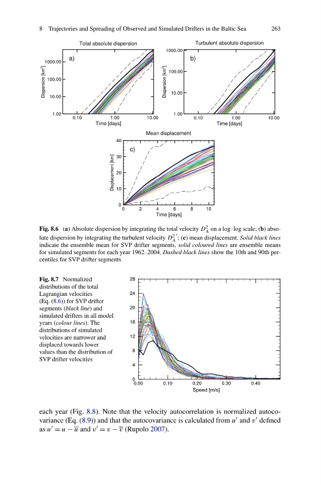
Fig. 8.6 (a) Absolute dispersion by integrating the total velocity D 2
A on a log–log scale; (b) absolute dispersion by integrating the turbulent velocity D 2
A
; (c) mean displacement. Solid black lines
indicate the ensemble mean for SVP drifter segments, solid coloured lines are ensemble means
for simulated segments for each year 1962–2004. Dashed black lines show the 10th and 90th percentiles for SVP drifter segments
Fig. 8.7 Normalized
distributions of the total
Lagrangian velocities
(Eq. (8.6)) for SVP drifter
segments (black line) and
simulated drifters in all model
years (colour lines). The
distributions of simulated
velocities are narrower and
displaced towards lower
values than the distribution of
SVP drifter velocities
each year (Fig. 8.8). Note that the velocity autocorrelation is normalized autocovariance (Eq. (8.9)) and that the autocovariance is calculated from u and v defined
as u = u − u and v = v − v (Rupolo 2007).
263
Fig. 8.6 (a) Absolute dispersion by integrating the total velocity D 2
A on a log–log scale; (b) absolute dispersion by integrating the turbulent velocity D 2
A
; (c) mean displacement. Solid black lines
indicate the ensemble mean for SVP drifter segments, solid coloured lines are ensemble means
for simulated segments for each year 1962–2004. Dashed black lines show the 10th and 90th percentiles for SVP drifter segments
Fig. 8.7 Normalized
distributions of the total
Lagrangian velocities
(Eq. (8.6)) for SVP drifter
segments (black line) and
simulated drifters in all model
years (colour lines). The
distributions of simulated
velocities are narrower and
displaced towards lower
values than the distribution of
SVP drifter velocities
each year (Fig. 8.8). Note that the velocity autocorrelation is normalized autocovariance (Eq. (8.9)) and that the autocovariance is calculated from u and v defined
as u = u − u and v = v − v (Rupolo 2007).