

7 TRACMASS—A Lagrangian Trajectory Model
237
has to be computed numerically for each direction. In the following subsection, we
describe how the roots s 1 and the corresponding exiting wall r 1 can be determined.
The displacement of the trajectory inside the considered grid box then proceeds as
discussed previously for stationary velocity fields.
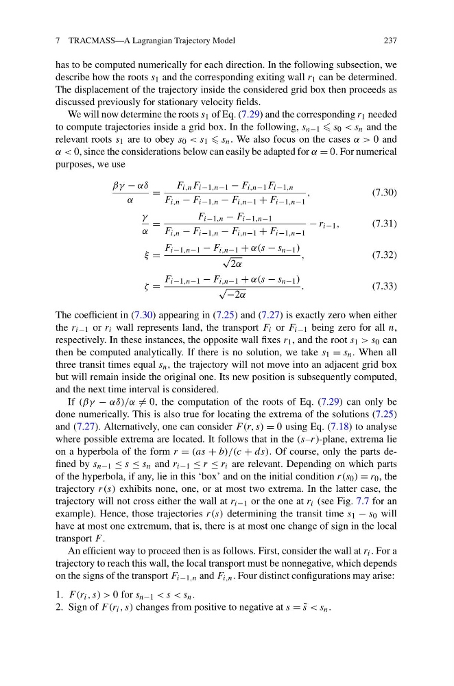
We will now determine the roots s 1 of Eq. (7.29) and the corresponding r 1 needed
to compute trajectories inside a grid box. In the following, s n−1 s 0 < s n and the
relevant roots s 1 are to obey s 0 < s 1 s n . We also focus on the cases α > 0 and
α < 0, since the considerations below can easily be adapted for α = 0. For numerical
purposes, we use
βγ − αδ
α
=
F i,n F i−1,n−1 − F i,n−1 F i−1,n
F i,n − F i−1,n − F i,n−1 + F i−1,n−1
,
(7.30)
γ
α
=
F i−1,n − F i−1,n−1
F i,n − F i−1,n − F i,n−1 + F i−1,n−1
− r i−1 ,
(7.31)
ξ =
F i−1,n−1 − F i,n−1 + α(s − s n−1 )
√
2α
,
(7.32)
ζ =
F i−1,n−1 − F i,n−1 + α(s − s n−1 )
√ −2α
.
(7.33)
The coefficient in (7.30) appearing in (7.25) and (7.27) is exactly zero when either
the r i−1 or r i wall represents land, the transport F i or F i−1 being zero for all n,
respectively. In these instances, the opposite wall fixes r 1 , and the root s 1 > s 0 can
then be computed analytically. If there is no solution, we take s 1 = s n . When all
three transit times equal s n , the trajectory will not move into an adjacent grid box
but will remain inside the original one. Its new position is subsequently computed,
and the next time interval is considered.
If (βγ − αδ)/α = 0, the computation of the roots of Eq. (7.29) can only be
done numerically. This is also true for locating the extrema of the solutions (7.25)
and (7.27). Alternatively, one can consider F (r, s) = 0 using Eq. (7.18) to analyse
where possible extrema are located. It follows that in the (s–r)-plane, extrema lie
on a hyperbola of the form r = (as + b)/(c + ds). Of course, only the parts defined by s n−1 ≤ s ≤ s n and r i−1 ≤ r ≤ r i are relevant. Depending on which parts
of the hyperbola, if any, lie in this ‘box’ and on the initial condition r(s 0 ) = r 0 , the
trajectory r(s) exhibits none, one, or at most two extrema. In the latter case, the
trajectory will not cross either the wall at r i−1 or the one at r i (see Fig. 7.7 for an
example). Hence, those trajectories r(s) determining the transit time s 1 − s 0 will
have at most one extremum, that is, there is at most one change of sign in the local
transport F .
An efficient way to proceed then is as follows. First, consider the wall at r i . For a
trajectory to reach this wall, the local transport must be nonnegative, which depends
on the signs of the transport F i−1,n and F i,n . Four distinct configurations may arise:
1. F (r i , s) > 0 for s n−1 < s < s n .
2. Sign of F (r i , s) changes from positive to negative at s = ˜
s < s n .
237
has to be computed numerically for each direction. In the following subsection, we
describe how the roots s 1 and the corresponding exiting wall r 1 can be determined.
The displacement of the trajectory inside the considered grid box then proceeds as
discussed previously for stationary velocity fields.
We will now determine the roots s 1 of Eq. (7.29) and the corresponding r 1 needed
to compute trajectories inside a grid box. In the following, s n−1 s 0 < s n and the
relevant roots s 1 are to obey s 0 < s 1 s n . We also focus on the cases α > 0 and
α < 0, since the considerations below can easily be adapted for α = 0. For numerical
purposes, we use
βγ − αδ
α
=
F i,n F i−1,n−1 − F i,n−1 F i−1,n
F i,n − F i−1,n − F i,n−1 + F i−1,n−1
,
(7.30)
γ
α
=
F i−1,n − F i−1,n−1
F i,n − F i−1,n − F i,n−1 + F i−1,n−1
− r i−1 ,
(7.31)
ξ =
F i−1,n−1 − F i,n−1 + α(s − s n−1 )
√
2α
,
(7.32)
ζ =
F i−1,n−1 − F i,n−1 + α(s − s n−1 )
√ −2α
.
(7.33)
The coefficient in (7.30) appearing in (7.25) and (7.27) is exactly zero when either
the r i−1 or r i wall represents land, the transport F i or F i−1 being zero for all n,
respectively. In these instances, the opposite wall fixes r 1 , and the root s 1 > s 0 can
then be computed analytically. If there is no solution, we take s 1 = s n . When all
three transit times equal s n , the trajectory will not move into an adjacent grid box
but will remain inside the original one. Its new position is subsequently computed,
and the next time interval is considered.
If (βγ − αδ)/α = 0, the computation of the roots of Eq. (7.29) can only be
done numerically. This is also true for locating the extrema of the solutions (7.25)
and (7.27). Alternatively, one can consider F (r, s) = 0 using Eq. (7.18) to analyse
where possible extrema are located. It follows that in the (s–r)-plane, extrema lie
on a hyperbola of the form r = (as + b)/(c + ds). Of course, only the parts defined by s n−1 ≤ s ≤ s n and r i−1 ≤ r ≤ r i are relevant. Depending on which parts
of the hyperbola, if any, lie in this ‘box’ and on the initial condition r(s 0 ) = r 0 , the
trajectory r(s) exhibits none, one, or at most two extrema. In the latter case, the
trajectory will not cross either the wall at r i−1 or the one at r i (see Fig. 7.7 for an
example). Hence, those trajectories r(s) determining the transit time s 1 − s 0 will
have at most one extremum, that is, there is at most one change of sign in the local
transport F .
An efficient way to proceed then is as follows. First, consider the wall at r i . For a
trajectory to reach this wall, the local transport must be nonnegative, which depends
on the signs of the transport F i−1,n and F i,n . Four distinct configurations may arise:
1. F (r i , s) > 0 for s n−1 < s < s n .
2. Sign of F (r i , s) changes from positive to negative at s = ˜
s < s n .