

238
K. Döös et al.
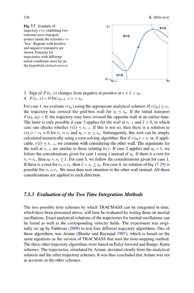
Fig. 7.7 Example of
trajectory r(s) exhibiting two
extrema (zero-transport
points) inside the relevant r–s
‘box.’ Regions with positive
and negative transports are
shown. Extrema for
trajectories with differing
initial conditions must lie on
the hyperbola (dotted curves)
3. Sign of F (r i , s) changes from negative to positive at s = ˆ
s < s n .
4. F (r i , s) < 0 for s n−1 < s < s n .
For case 1, we evaluate r(s n ) using the appropriate analytical solution. If r(s n ) ≥ r i ,
the trajectory has crossed the grid-box wall for s 1 ≤ s n . If the initial transport
F (r 0 , s 0 ) < 0, the trajectory may have crossed the opposite wall at an earlier time.
The latter is only possible if case 3 applies for the wall at r i−1 and ˆ
s > 0, in which
case one checks whether r(ˆ s) ≤ r i−1 . If this is not so, then there is a solution to
r(s 1 ) − r 1 = 0 for r 1 = r i and s 0 < s 1 ≤ s n . Subsequently, this root can be simply
calculated numerically using a root-solving algorithm. But if r(s n ) < r i or, if applicable, r(ˆ s) ≤ r i−1 , we continue with considering the other wall. The arguments for
the wall at r i−1 are similar to those relating to r. If case 2 applies and s 0 < ˜
s, we
follow the considerations given for case 1 using ˜
s instead of s n . If there is a root for
r 1 = r i , then s 0 < s 1 ≤ ˆ
s. For case 3, we follow the considerations given for case 1.
If there is a root for r 1 = r i , then ˆ
s < s 1 ≤ s n . For case 4, no solution of Eq. (7.29) is
possible for r 1 = r i . We must then turn attention to the other wall instead. All these
considerations are applied to each direction.
7.5.3 Evaluation of the Two Time Integration Methods
The two possible time schemes by which TRACMASS can be integrated in time,
which have been presented above, will here be evaluated by testing them on inertial
oscillations. Exact analytical solutions of the trajectories for inertial oscillations can
be found as well as the corresponding velocity fields. The experiment was originally set up by Fabbroni (2009) to test four different trajectory algorithms. One of
these algorithms was Ariane (Blanke and Raynaud 1997), which is based on the
same equations as the version of TRACMASS that uses the time-stepping method.
The three other trajectory algorithms were based on Euler forward and Runge–Kutta
schemes. The trajectories, simulated by Ariane, deviated clearly from the analytical
solution and the other trajectory schemes. It was thus concluded that Ariane was not
as accurate as the other schemes.
K. Döös et al.
Fig. 7.7 Example of
trajectory r(s) exhibiting two
extrema (zero-transport
points) inside the relevant r–s
‘box.’ Regions with positive
and negative transports are
shown. Extrema for
trajectories with differing
initial conditions must lie on
the hyperbola (dotted curves)
3. Sign of F (r i , s) changes from negative to positive at s = ˆ
s < s n .
4. F (r i , s) < 0 for s n−1 < s < s n .
For case 1, we evaluate r(s n ) using the appropriate analytical solution. If r(s n ) ≥ r i ,
the trajectory has crossed the grid-box wall for s 1 ≤ s n . If the initial transport
F (r 0 , s 0 ) < 0, the trajectory may have crossed the opposite wall at an earlier time.
The latter is only possible if case 3 applies for the wall at r i−1 and ˆ
s > 0, in which
case one checks whether r(ˆ s) ≤ r i−1 . If this is not so, then there is a solution to
r(s 1 ) − r 1 = 0 for r 1 = r i and s 0 < s 1 ≤ s n . Subsequently, this root can be simply
calculated numerically using a root-solving algorithm. But if r(s n ) < r i or, if applicable, r(ˆ s) ≤ r i−1 , we continue with considering the other wall. The arguments for
the wall at r i−1 are similar to those relating to r. If case 2 applies and s 0 < ˜
s, we
follow the considerations given for case 1 using ˜
s instead of s n . If there is a root for
r 1 = r i , then s 0 < s 1 ≤ ˆ
s. For case 3, we follow the considerations given for case 1.
If there is a root for r 1 = r i , then ˆ
s < s 1 ≤ s n . For case 4, no solution of Eq. (7.29) is
possible for r 1 = r i . We must then turn attention to the other wall instead. All these
considerations are applied to each direction.
7.5.3 Evaluation of the Two Time Integration Methods
The two possible time schemes by which TRACMASS can be integrated in time,
which have been presented above, will here be evaluated by testing them on inertial
oscillations. Exact analytical solutions of the trajectories for inertial oscillations can
be found as well as the corresponding velocity fields. The experiment was originally set up by Fabbroni (2009) to test four different trajectory algorithms. One of
these algorithms was Ariane (Blanke and Raynaud 1997), which is based on the
same equations as the version of TRACMASS that uses the time-stepping method.
The three other trajectory algorithms were based on Euler forward and Runge–Kutta
schemes. The trajectories, simulated by Ariane, deviated clearly from the analytical
solution and the other trajectory schemes. It was thus concluded that Ariane was not
as accurate as the other schemes.