

236
K. Döös et al.
where t G is the time step between two data sets in true time dimension (seconds).
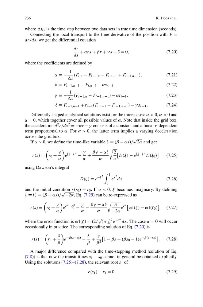
Connecting the local transport to the time derivative of the position with F =
dr/ds, we get the differential equation
dr
ds
+ αrs + βr + γ s + δ = 0,
(7.20)
where the coefficients are defined by
α ≡ −
1
s
(F i,n − F i−1,n − F i,n−1 + F i−1,n−1 ),
(7.21)
β ≡ F i−1,n−1 − F i,n−1 − αs n−1 ,
(7.22)
γ ≡ −
1
s
(F i−1,n − F i−1,n−1 ) − αr i−1 ,
(7.23)
δ ≡ F i−1,n−1 + r i−1 (F i,n−1 − F i−1,n−1 ) − γ s n−1 .
(7.24)
Differently shaped analytical solutions exist for the three cases: α > 0, α < 0 and
α = 0, which together cover all possible values of α. Note that inside the grid box,
the acceleration d 2 r/ds 2 = −αr − γ consists of a constant and a linear r-dependent
term proportional to α. For α > 0, the latter term implies a varying deceleration
across the grid box.
If α > 0, we define the time-like variable ξ = (β + αs)/
√
2α and get
r(s) =
r 0 +
γ
α
e
ξ 2
0 −ξ 2 −
γ
α
+
βγ − αδ
α
2
α
D(ξ ) − e
ξ 2
0 −ξ 2
D(ξ 0 )
(7.25)
using Dawson’s integral
D(ξ ) ≡ e
−ξ 2
ξ
0
e
x 2
dx
(7.26)
and the initial condition r(s 0 ) = r 0 . If α < 0, ξ becomes imaginary. By defining
ζ ≡ iξ = (β + αs)/
√ −2α, Eq. (7.25) can be re-expressed as
r(s) =
r 0 +
γ
α
e
ζ 2 −ζ 2
0 −
γ
α
−
βγ − αδ
α
π
−2α
e
ζ 2
erf(ζ ) − erf(ζ 0 )
, (7.27)
where the error function is erf(ζ ) = (2/
√
)π
ζ
0 e −x 2 dx. The case α = 0 will occur
occasionally in practice. The corresponding solution of Eq. (7.20) is
r(s) =
r 0 +
δ
β
e
−β(s−s 0 )
−
δ
β
+
γ
β 2
1 − βs + (βs 0 − 1)e
−β(s−s 0 )
. (7.28)
A major difference compared with the time-stepping method (solution of Eq.
(7.8)) is that now the transit times s 1 − s 0 cannot in general be obtained explicitly.
Using the solutions (7.25)–(7.28), the relevant root s 1 of
r(s 1 ) − r 1 = 0
(7.29)
K. Döös et al.
where t G is the time step between two data sets in true time dimension (seconds).
Connecting the local transport to the time derivative of the position with F =
dr/ds, we get the differential equation
dr
ds
+ αrs + βr + γ s + δ = 0,
(7.20)
where the coefficients are defined by
α ≡ −
1
s
(F i,n − F i−1,n − F i,n−1 + F i−1,n−1 ),
(7.21)
β ≡ F i−1,n−1 − F i,n−1 − αs n−1 ,
(7.22)
γ ≡ −
1
s
(F i−1,n − F i−1,n−1 ) − αr i−1 ,
(7.23)
δ ≡ F i−1,n−1 + r i−1 (F i,n−1 − F i−1,n−1 ) − γ s n−1 .
(7.24)
Differently shaped analytical solutions exist for the three cases: α > 0, α < 0 and
α = 0, which together cover all possible values of α. Note that inside the grid box,
the acceleration d 2 r/ds 2 = −αr − γ consists of a constant and a linear r-dependent
term proportional to α. For α > 0, the latter term implies a varying deceleration
across the grid box.
If α > 0, we define the time-like variable ξ = (β + αs)/
√
2α and get
r(s) =
r 0 +
γ
α
e
ξ 2
0 −ξ 2 −
γ
α
+
βγ − αδ
α
2
α
D(ξ ) − e
ξ 2
0 −ξ 2
D(ξ 0 )
(7.25)
using Dawson’s integral
D(ξ ) ≡ e
−ξ 2
ξ
0
e
x 2
dx
(7.26)
and the initial condition r(s 0 ) = r 0 . If α < 0, ξ becomes imaginary. By defining
ζ ≡ iξ = (β + αs)/
√ −2α, Eq. (7.25) can be re-expressed as
r(s) =
r 0 +
γ
α
e
ζ 2 −ζ 2
0 −
γ
α
−
βγ − αδ
α
π
−2α
e
ζ 2
erf(ζ ) − erf(ζ 0 )
, (7.27)
where the error function is erf(ζ ) = (2/
√
)π
ζ
0 e −x 2 dx. The case α = 0 will occur
occasionally in practice. The corresponding solution of Eq. (7.20) is
r(s) =
r 0 +
δ
β
e
−β(s−s 0 )
−
δ
β
+
γ
β 2
1 − βs + (βs 0 − 1)e
−β(s−s 0 )
. (7.28)
A major difference compared with the time-stepping method (solution of Eq.
(7.8)) is that now the transit times s 1 − s 0 cannot in general be obtained explicitly.
Using the solutions (7.25)–(7.28), the relevant root s 1 of
r(s 1 ) − r 1 = 0
(7.29)