

234
K. Döös et al.
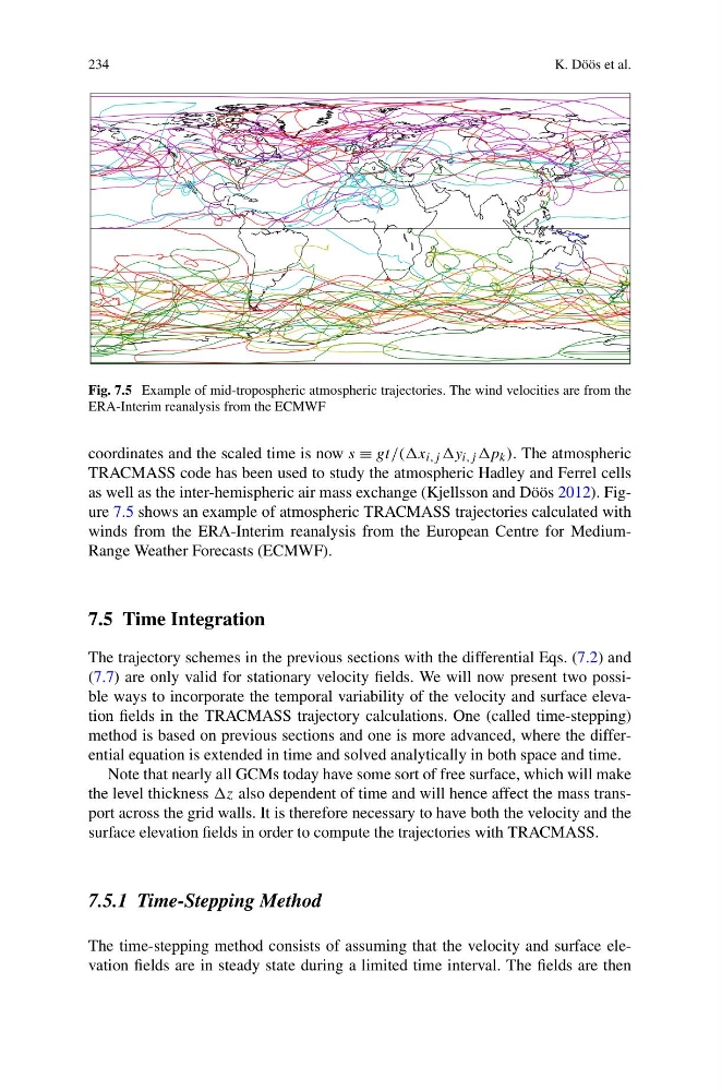
Fig. 7.5 Example of mid-tropospheric atmospheric trajectories. The wind velocities are from the
ERA-Interim reanalysis from the ECMWF
coordinates and the scaled time is now s ≡ gt/((x i,j y i,j p k ). The atmospheric
TRACMASS code has been used to study the atmospheric Hadley and Ferrel cells
as well as the inter-hemispheric air mass exchange (Kjellsson and Döös 2012). Figure 7.5 shows an example of atmospheric TRACMASS trajectories calculated with
winds from the ERA-Interim reanalysis from the European Centre for MediumRange Weather Forecasts (ECMWF).
7.5 Time Integration
The trajectory schemes in the previous sections with the differential Eqs. (7.2) and
(7.7) are only valid for stationary velocity fields. We will now present two possible ways to incorporate the temporal variability of the velocity and surface elevation fields in the TRACMASS trajectory calculations. One (called time-stepping)
method is based on previous sections and one is more advanced, where the differential equation is extended in time and solved analytically in both space and time.
Note that nearly all GCMs today have some sort of free surface, which will make
the level thickness z also dependent of time and will hence affect the mass transport across the grid walls. It is therefore necessary to have both the velocity and the
surface elevation fields in order to compute the trajectories with TRACMASS.
7.5.1 Time-Stepping Method
The time-stepping method consists of assuming that the velocity and surface elevation fields are in steady state during a limited time interval. The fields are then
K. Döös et al.
Fig. 7.5 Example of mid-tropospheric atmospheric trajectories. The wind velocities are from the
ERA-Interim reanalysis from the ECMWF
coordinates and the scaled time is now s ≡ gt/((x i,j y i,j p k ). The atmospheric
TRACMASS code has been used to study the atmospheric Hadley and Ferrel cells
as well as the inter-hemispheric air mass exchange (Kjellsson and Döös 2012). Figure 7.5 shows an example of atmospheric TRACMASS trajectories calculated with
winds from the ERA-Interim reanalysis from the European Centre for MediumRange Weather Forecasts (ECMWF).
7.5 Time Integration
The trajectory schemes in the previous sections with the differential Eqs. (7.2) and
(7.7) are only valid for stationary velocity fields. We will now present two possible ways to incorporate the temporal variability of the velocity and surface elevation fields in the TRACMASS trajectory calculations. One (called time-stepping)
method is based on previous sections and one is more advanced, where the differential equation is extended in time and solved analytically in both space and time.
Note that nearly all GCMs today have some sort of free surface, which will make
the level thickness z also dependent of time and will hence affect the mass transport across the grid walls. It is therefore necessary to have both the velocity and the
surface elevation fields in order to compute the trajectories with TRACMASS.
7.5.1 Time-Stepping Method
The time-stepping method consists of assuming that the velocity and surface elevation fields are in steady state during a limited time interval. The fields are then