

7 TRACMASS—A Lagrangian Trajectory Model
233
is the surface pressure. The dependent variables, which are the zonal wind u, the
meridional wind v, the temperature T and the specific humidity q are defined in the
middle of the layers, where the pressure is defined by p k =
1
2 (p k−1/2 + p k+1/2 ), for
k = 1, 2, . . . , N LEV . The vertical coordinate is η = η(p, p S ) and has the boundary
value η(0, p S ) = 0 at the top of the atmosphere and η(p S , p S ) = 1 at the Earth’s
surface.
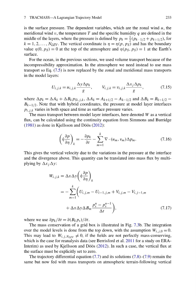
For the ocean, in the previous sections, we used volume transport because of the
incompressibility approximation. In the atmosphere we need instead to use mass
transport so Eq. (7.5) is now replaced by the zonal and meridional mass transports
in the model layers:
U i,j,k = u i,j,k
k
g
,
V i,j,k = v i,j,k
x j p k
g
,
(7.15)
where p k = A k + B k p Si,j,k , A k = A k+1/2 − A k−1/2 and B k = B k+1/2 −
B k−1/2 . Note that with hybrid coordinates, the pressure at model layer interfaces
p i,j,k varies in both space and time as surface pressure varies.
The mass transport between model layer interfaces, here denoted W as a vertical
flux, can be calculated using the continuity equation from Simmons and Burridge
(1981) as done in Kjellsson and Döös (2012):
˙
η
∂p
∂η
k
= −
∂p k
∂t
−
k
m=1
∇ · (u m , v m ))p m .
(7.16)
This gives the vertical velocity due to the variations in the pressure at the interface
and the divergence above. This quantity can be translated into mass flux by multiplying by x j y:
W i,j,k =
˙
η
∂p
∂η
k
= −
k
m=1
U i,j,m − U i−1,j,m + V i,j,m − V i,j −1,m
+ m
p n
s − p n−1
s
t
,
(7.17)
where we use ∂p k /∂t = ∂(B k p s )/∂t.
The mass conservation of a grid box is illustrated in Fig. 7.3b. The integration
over the model levels is done from the top down, with the assumption W i,j,0 = 0.
This may lead to W i,j,N LEV = 0, if the fields are not perfectly mass-conserving,
which is the case for reanalysis data (see Berrisford et al. 2011 for a study on ERAInterim) as used by Kjellsson and Döös (2012). In such a case, the vertical flux at
the surface must be explicitly set to zero.
The trajectory differential equation (7.7) and its solutions (7.8)–(7.9) remain the
same but now fed with mass transports on atmospheric terrain-following vertical
233
is the surface pressure. The dependent variables, which are the zonal wind u, the
meridional wind v, the temperature T and the specific humidity q are defined in the
middle of the layers, where the pressure is defined by p k =
1
2 (p k−1/2 + p k+1/2 ), for
k = 1, 2, . . . , N LEV . The vertical coordinate is η = η(p, p S ) and has the boundary
value η(0, p S ) = 0 at the top of the atmosphere and η(p S , p S ) = 1 at the Earth’s
surface.
For the ocean, in the previous sections, we used volume transport because of the
incompressibility approximation. In the atmosphere we need instead to use mass
transport so Eq. (7.5) is now replaced by the zonal and meridional mass transports
in the model layers:
U i,j,k = u i,j,k
k
g
,
V i,j,k = v i,j,k
x j p k
g
,
(7.15)
where p k = A k + B k p Si,j,k , A k = A k+1/2 − A k−1/2 and B k = B k+1/2 −
B k−1/2 . Note that with hybrid coordinates, the pressure at model layer interfaces
p i,j,k varies in both space and time as surface pressure varies.
The mass transport between model layer interfaces, here denoted W as a vertical
flux, can be calculated using the continuity equation from Simmons and Burridge
(1981) as done in Kjellsson and Döös (2012):
˙
η
∂p
∂η
k
= −
∂p k
∂t
−
k
m=1
∇ · (u m , v m ))p m .
(7.16)
This gives the vertical velocity due to the variations in the pressure at the interface
and the divergence above. This quantity can be translated into mass flux by multiplying by x j y:
W i,j,k =
˙
η
∂p
∂η
k
= −
k
m=1
U i,j,m − U i−1,j,m + V i,j,m − V i,j −1,m
+ m
p n
s − p n−1
s
t
,
(7.17)
where we use ∂p k /∂t = ∂(B k p s )/∂t.
The mass conservation of a grid box is illustrated in Fig. 7.3b. The integration
over the model levels is done from the top down, with the assumption W i,j,0 = 0.
This may lead to W i,j,N LEV = 0, if the fields are not perfectly mass-conserving,
which is the case for reanalysis data (see Berrisford et al. 2011 for a study on ERAInterim) as used by Kjellsson and Döös (2012). In such a case, the vertical flux at
the surface must be explicitly set to zero.
The trajectory differential equation (7.7) and its solutions (7.8)–(7.9) remain the
same but now fed with mass transports on atmospheric terrain-following vertical