

7 TRACMASS—A Lagrangian Trajectory Model
231
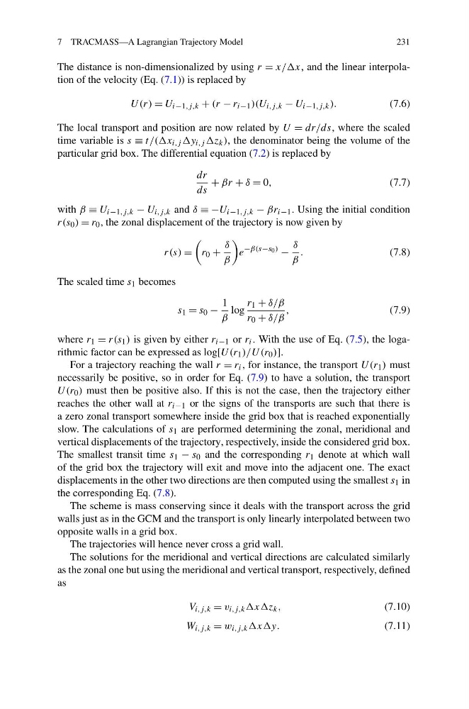
The distance is non-dimensionalized by using r = x//x, and the linear interpolation of the velocity (Eq. (7.1)) is replaced by
U(r) = U i−1,j,k + (r − r i−1 )(U i,j,k − U i−1,j,k ).
(7.6)
The local transport and position are now related by U = dr/ds, where the scaled
time variable is s ≡ t/((x i,j y i,j z k ), the denominator being the volume of the
particular grid box. The differential equation (7.2) is replaced by
dr
ds
+ βr + δ = 0,
(7.7)
with β ≡ U i−1,j,k − U i,j,k and δ ≡ −U i−1,j,k − βr i−1 . Using the initial condition
r(s 0 ) = r 0 , the zonal displacement of the trajectory is now given by
r(s) =
r 0 +
δ
β
e
−β(s−s 0 )
−
δ
β
.
(7.8)
The scaled time s 1 becomes
s 1 = s 0 −
1
β
log
r 1 + δ/β
r 0 + δ/β
,
(7.9)
where r 1 = r(s 1 ) is given by either r i−1 or r i . With the use of Eq. (7.5), the logarithmic factor can be expressed as log[U(r 1 )/U (r 0 )].
For a trajectory reaching the wall r = r i , for instance, the transport U(r 1 ) must
necessarily be positive, so in order for Eq. (7.9) to have a solution, the transport
U(r 0 ) must then be positive also. If this is not the case, then the trajectory either
reaches the other wall at r i−1 or the signs of the transports are such that there is
a zero zonal transport somewhere inside the grid box that is reached exponentially
slow. The calculations of s 1 are performed determining the zonal, meridional and
vertical displacements of the trajectory, respectively, inside the considered grid box.
The smallest transit time s 1 − s 0 and the corresponding r 1 denote at which wall
of the grid box the trajectory will exit and move into the adjacent one. The exact
displacements in the other two directions are then computed using the smallest s 1 in
the corresponding Eq. (7.8).
The scheme is mass conserving since it deals with the transport across the grid
walls just as in the GCM and the transport is only linearly interpolated between two
opposite walls in a grid box.
The trajectories will hence never cross a grid wall.
The solutions for the meridional and vertical directions are calculated similarly
as the zonal one but using the meridional and vertical transport, respectively, defined
as
V i,j,k = v i,j,k k ,
(7.10)
W i,j,k = w i,j,k
(7.11)
231
The distance is non-dimensionalized by using r = x//x, and the linear interpolation of the velocity (Eq. (7.1)) is replaced by
U(r) = U i−1,j,k + (r − r i−1 )(U i,j,k − U i−1,j,k ).
(7.6)
The local transport and position are now related by U = dr/ds, where the scaled
time variable is s ≡ t/((x i,j y i,j z k ), the denominator being the volume of the
particular grid box. The differential equation (7.2) is replaced by
dr
ds
+ βr + δ = 0,
(7.7)
with β ≡ U i−1,j,k − U i,j,k and δ ≡ −U i−1,j,k − βr i−1 . Using the initial condition
r(s 0 ) = r 0 , the zonal displacement of the trajectory is now given by
r(s) =
r 0 +
δ
β
e
−β(s−s 0 )
−
δ
β
.
(7.8)
The scaled time s 1 becomes
s 1 = s 0 −
1
β
log
r 1 + δ/β
r 0 + δ/β
,
(7.9)
where r 1 = r(s 1 ) is given by either r i−1 or r i . With the use of Eq. (7.5), the logarithmic factor can be expressed as log[U(r 1 )/U (r 0 )].
For a trajectory reaching the wall r = r i , for instance, the transport U(r 1 ) must
necessarily be positive, so in order for Eq. (7.9) to have a solution, the transport
U(r 0 ) must then be positive also. If this is not the case, then the trajectory either
reaches the other wall at r i−1 or the signs of the transports are such that there is
a zero zonal transport somewhere inside the grid box that is reached exponentially
slow. The calculations of s 1 are performed determining the zonal, meridional and
vertical displacements of the trajectory, respectively, inside the considered grid box.
The smallest transit time s 1 − s 0 and the corresponding r 1 denote at which wall
of the grid box the trajectory will exit and move into the adjacent one. The exact
displacements in the other two directions are then computed using the smallest s 1 in
the corresponding Eq. (7.8).
The scheme is mass conserving since it deals with the transport across the grid
walls just as in the GCM and the transport is only linearly interpolated between two
opposite walls in a grid box.
The trajectories will hence never cross a grid wall.
The solutions for the meridional and vertical directions are calculated similarly
as the zonal one but using the meridional and vertical transport, respectively, defined
as
V i,j,k = v i,j,k k ,
(7.10)
W i,j,k = w i,j,k
(7.11)