

230
K. Döös et al.
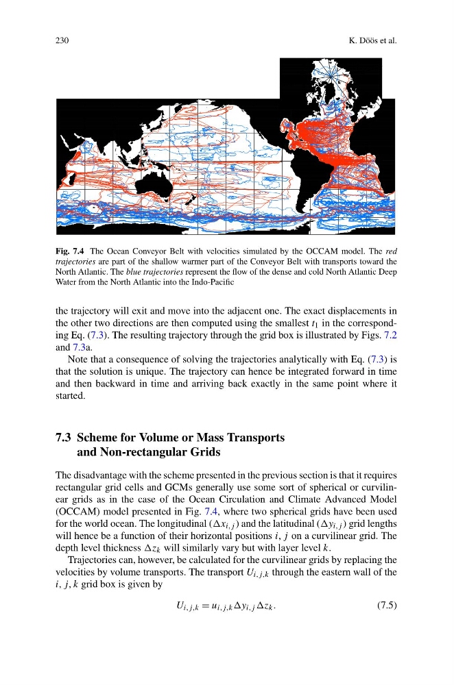
Fig. 7.4 The Ocean Conveyor Belt with velocities simulated by the OCCAM model. The red
trajectories are part of the shallow warmer part of the Conveyor Belt with transports toward the
North Atlantic. The blue trajectories represent the flow of the dense and cold North Atlantic Deep
Water from the North Atlantic into the Indo-Pacific
the trajectory will exit and move into the adjacent one. The exact displacements in
the other two directions are then computed using the smallest t 1 in the corresponding Eq. (7.3). The resulting trajectory through the grid box is illustrated by Figs. 7.2
and 7.3a.
Note that a consequence of solving the trajectories analytically with Eq. (7.3) is
that the solution is unique. The trajectory can hence be integrated forward in time
and then backward in time and arriving back exactly in the same point where it
started.
7.3 Scheme for Volume or Mass Transports
and Non-rectangular Grids
The disadvantage with the scheme presented in the previous section is that it requires
rectangular grid cells and GCMs generally use some sort of spherical or curvilinear grids as in the case of the Ocean Circulation and Climate Advanced Model
(OCCAM) model presented in Fig. 7.4, where two spherical grids have been used
for the world ocean. The longitudinal (x i,j ) and the latitudinal (y i,j ) grid lengths
will hence be a function of their horizontal positions i, j on a curvilinear grid. The
depth level thickness z k will similarly vary but with layer level k.
Trajectories can, however, be calculated for the curvilinear grids by replacing the
velocities by volume transports. The transport U i,j,k through the eastern wall of the
i, j, k grid box is given by
U i,j,k = u i,j,k y i,j z k .
(7.5)
K. Döös et al.
Fig. 7.4 The Ocean Conveyor Belt with velocities simulated by the OCCAM model. The red
trajectories are part of the shallow warmer part of the Conveyor Belt with transports toward the
North Atlantic. The blue trajectories represent the flow of the dense and cold North Atlantic Deep
Water from the North Atlantic into the Indo-Pacific
the trajectory will exit and move into the adjacent one. The exact displacements in
the other two directions are then computed using the smallest t 1 in the corresponding Eq. (7.3). The resulting trajectory through the grid box is illustrated by Figs. 7.2
and 7.3a.
Note that a consequence of solving the trajectories analytically with Eq. (7.3) is
that the solution is unique. The trajectory can hence be integrated forward in time
and then backward in time and arriving back exactly in the same point where it
started.
7.3 Scheme for Volume or Mass Transports
and Non-rectangular Grids
The disadvantage with the scheme presented in the previous section is that it requires
rectangular grid cells and GCMs generally use some sort of spherical or curvilinear grids as in the case of the Ocean Circulation and Climate Advanced Model
(OCCAM) model presented in Fig. 7.4, where two spherical grids have been used
for the world ocean. The longitudinal (x i,j ) and the latitudinal (y i,j ) grid lengths
will hence be a function of their horizontal positions i, j on a curvilinear grid. The
depth level thickness z k will similarly vary but with layer level k.
Trajectories can, however, be calculated for the curvilinear grids by replacing the
velocities by volume transports. The transport U i,j,k through the eastern wall of the
i, j, k grid box is given by
U i,j,k = u i,j,k y i,j z k .
(7.5)